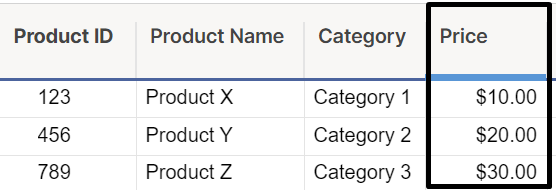
Have you ever needed to pull a value from a range based on a matching value in your list? For example, you may want to dynamically pull the price of a product based on the product’s ID.
If your data set contains the Product ID, you can use a formula to pull the price.
With this formula set as a column formula, each row (and any newly added rows) will show the matching price from the product data set.
Different approaches to this formula
There are three methods you can use to pull data from a range based on a matching lookup value:
VLOOKUP
INDEX(MATCH())
INDEX(COLLECT())
We’ll review how to use each of these formulas, as well as discuss pros and cons to each approach.
VLOOKUP
A VLOOKUP formula looks up a value and returns a value in the same row, but from a different (specified) column. The format for a VLOOKUP formula can be found below:
=VLOOKUP([Lookup value], [Data set being searched], [Column number in data set],[False or true based on exact match needs])
To pull the price in the example above using a VLOOKUP, your formula would look like this:
=VLOOKUP([Associated Product ID]@row, {Product Data | Product}, 4, false)
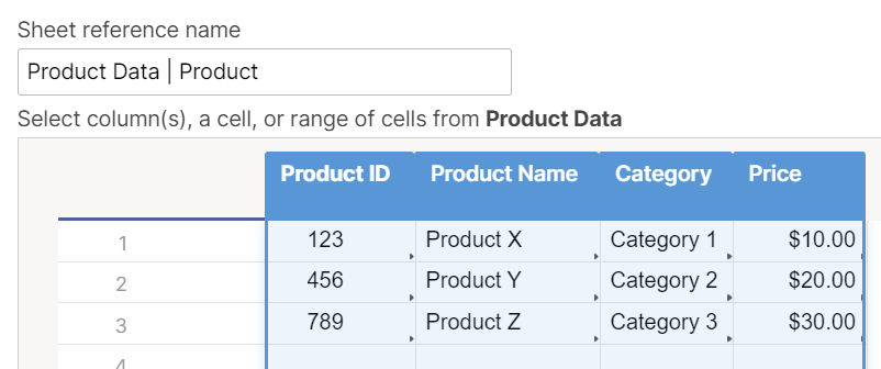
The {Product Data | Product} cross-sheet reference range looks like this:
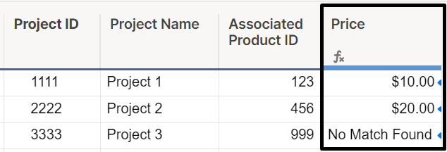
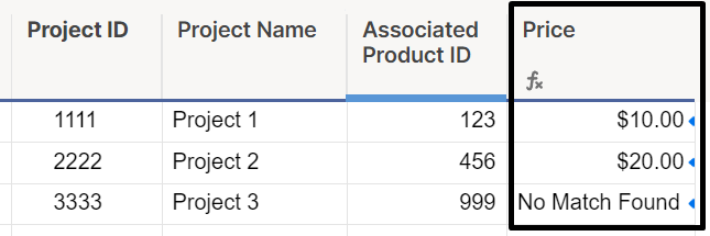
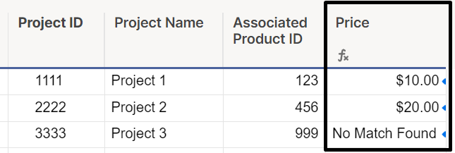
And the formula returns the values in the Price column like this:
TIP: Wrap the formula with an IFERROR formula to solve for cases where no match is found in the data set being searched. In this example, the formula would look like:
=IFERROR(VLOOKUP([Associated Product ID]@row, {Product Data | Product}, 4, false), "No Match Found")
Pros:
Simple/quickest formula
Cons:
Requires lookup value to be first column in data set being searched
Unable to pull values to the left of the lookup value column
Breaks if a new column is added or column is removed between lookup value and column being pulled in, or if columns are reordered
INDEX(MATCH())
An INDEX(MATCH()) formula searches a range and collects the value that matches the criteria specified. The format for an INDEX(MATCH()) formula can be found below:
=INDEX([Range with value to be returned],MATCH([Search value],[Range with value being searched],[0, 1, or -1 depending on search type]))
To pull the price in the example above using an INDEX(MATCH()), your formula would look like this:
=IFERROR(INDEX({Product Data | Price}, MATCH([Associated Product ID]@row, {Product Data | Product ID}, 0)), "No Match Found")
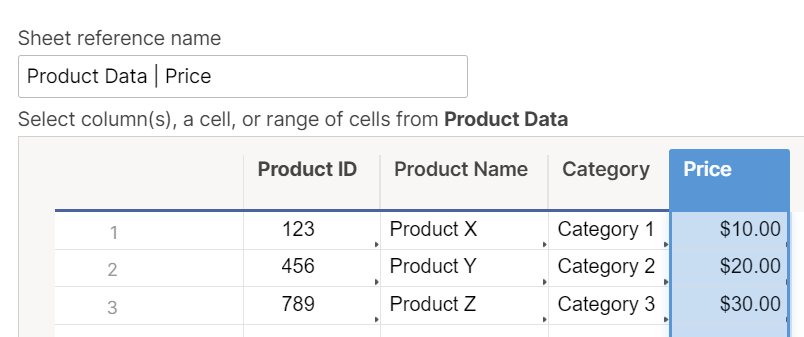
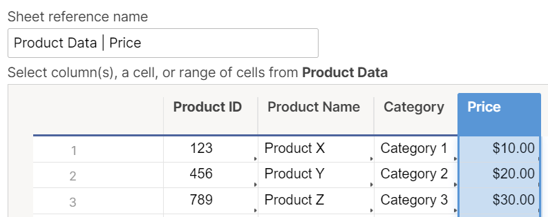
The {Product Data | Price} cross-sheet reference range looks like this:
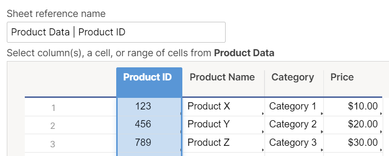
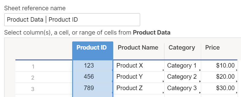
The {Product Data | Product ID} cross-sheet reference range looks like this:
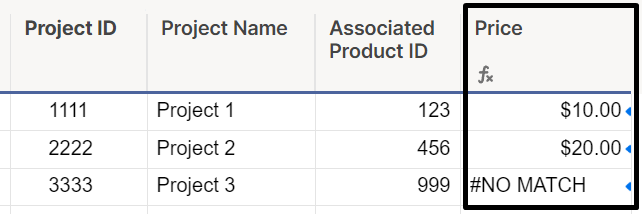
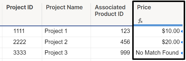
As noted above, we’ve also wrapped our INDEX(MATCH()) function in an IFERROR to show “No Match Found” if no matching Product ID is found for the row, so the formula returns the values in the Price column like this:
Pros:
Allows for changes to ordering of columns or deleting unused columns without breaking
Can pull values from columns to left or right of search value range
Faster for larger data sets
INDEX(MATCH(),MATCH()) can be used for dynamic matching of columns and rows
The total number of referenced cells is usually lower, helping to keep you away from the 100,000 total limit of cells referenced in cross-sheet references.
Cons:
Requires more than one cross-sheet reference for cases where reference data exists in a separate sheet
Limited to a single match criteria
INDEX(COLLECT())
An INDEX(COLLECT()) formula searches a range and collects the value that matches one or more criteria specified. The format for an INDEX(COLLECT()) formula can be found below:
=INDEX(COLLECT([Range with value to be returned],[Range with criterion],[Criterion],[Range 2 with criterion],[Criterion], etc.),[1 for row index to be returned])
To pull the price in the example above using an INDEX(COLLECT()), your formula would look like this:
=IFERROR(INDEX(COLLECT({Product Data | Price}, {Product Data | Product ID}, [Associated Product ID]@row), 1), "No Match Found")
The {Product Data | Price} cross-sheet reference range looks like this:
The {Product Data | Product ID} cross-sheet reference range looks like this:
As noted above, we’ve also wrapped our INDEX(COLLECT()) function in an IFERROR to show “No Match Found” if no matching Product ID is found for the row, so the formula returns the values in the Price column like this:
Pros:
Allows for changes to ordering of columns or deleting unused columns without breaking
Can pull values from columns to left or right of search value range
Usually faster than VLOOKUP, but may be slower than INDEX/MATCH.
Allows for multiple criteria to be used within COLLECT formula to match on multiple columns or create more complex criteria.
Allows you to provide the second, third, etc. matches by replacing the “, 1” at the end of the formula instead of always providing the first match.
Cons:
Requires more than one cross-sheet reference for cases where reference data exists in a separate sheet.
May be slower than using an INDEX/MATCH, especially if using multiple criteria.
Still need help?
Use the Formula Handbook template to find more support resources, and view 100+ formulas, including a glossary of every function that you can practice working with in real time, and examples of commonly used and advanced formulas.
Find examples of how other Smartsheet customers use this function or ask about your specific use case in the Smartsheet Community. Ask the Community