What Is Conditional Formatting?
Conditional formatting is a feature of many spreadsheet applications that allows you to apply special formatting to cells that meet certain criteria. It is most often used to highlight, emphasize, or differentiate among data and information stored in a spreadsheet.
Conditional formatting enables spreadsheet users to do a number of things. First and foremost, it calls attention to important data points such as deadlines, at-risk tasks, or budget items. It can also make large data sets more digestible by breaking up the wall of numbers with a visual organizational component. Finally, conditional formatting can transform your spreadsheet (that previously only stored data) into a dependable “alert” system that highlights key information and keeps you on top of your workload.
Originally a powerful feature of Excel, other spreadsheet applications have also adopted this functionality.
Conditional Formatting Basics
Conditional formatting consists of four main components: if-then commands, preset conditions, custom conditions, and applying multiple conditions. We’ve outlined how to use these commands and conditions to create and apply rules to your Excel spreadsheets below:
- If-Then Logic: All conditional formatting rules are based on simple if-then logic: if X criteria is true, then Y formatting will be applied (this is often written as p → q, or if p is true, then apply q). You won’t have to hard-code any logic, though - Excel and other spreadsheet apps have built-in parameters so you can simply select the conditions you want the rules to meet. Advanced users can also apply the program’s built-in formulas to logic rules.
- Preset Conditions: Excel has a huge library of preset rules encompassing nearly all functions that beginner users will want to apply. We’ll familiarize you with several of the most popular ones in the next section.
- Custom Conditions: For situations where you want to manipulate a preset condition, you can create your own rules. If appropriate, you can use Excel formulas in the rules you write.
- Applying Multiple Conditions: You can apply multiple rules to a single cell or range of cells. However, be aware of rule hierarchy and precedence - we’ll show you how to manage stacked rules in the walkthrough.
Overall, applying conditional formatting is an easy way to keep you and your team members up to date with your data - calling visual attention to important dates and deadlines, tasks and assignments, budget constraints, and anything else you might want to highlight. When applied correctly, conditional formatting will make you more productive by reducing time spent manually combing data and making it easier to identify trends, so you can focus on the big decisions.
How to Apply Basic Conditional Formatting in Excel
You can apply conditional formatting to your Excel spreadsheets using various tools and features found within the program. This step-by-step walkthrough shows you how to apply the most commonly used formatting for highlighting, data bars, color scales, and more.
Step 1: Apply Highlight Rules to Your Excel Spreadsheet
Highlight rules apply color formatting to cells that meet specific criteria that you define. They are the most basic type of conditional formatting rule, and Excel provides a variety of preset highlight functions.
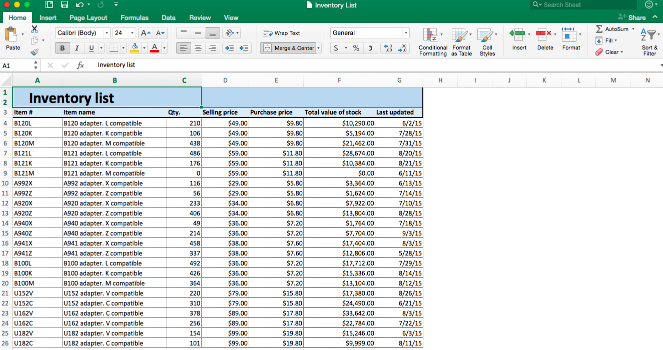
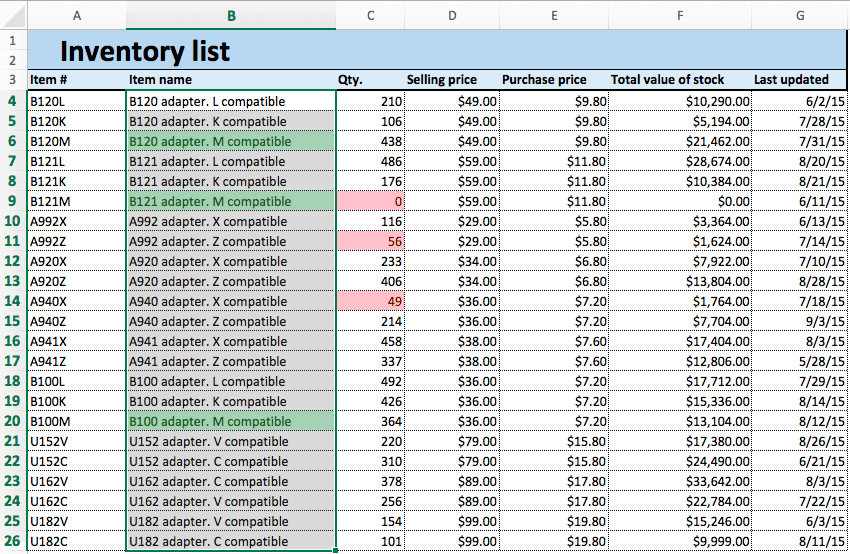
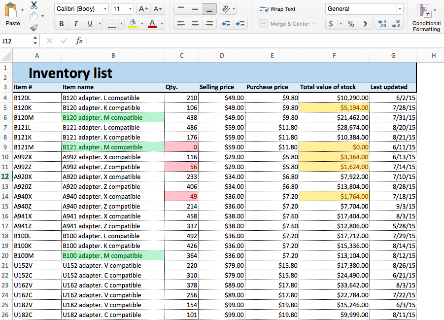
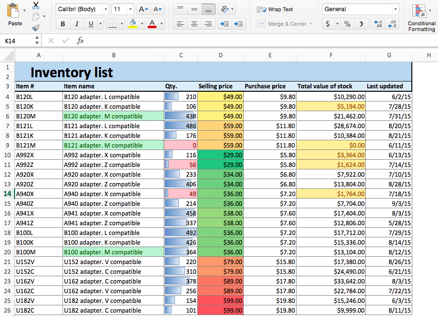
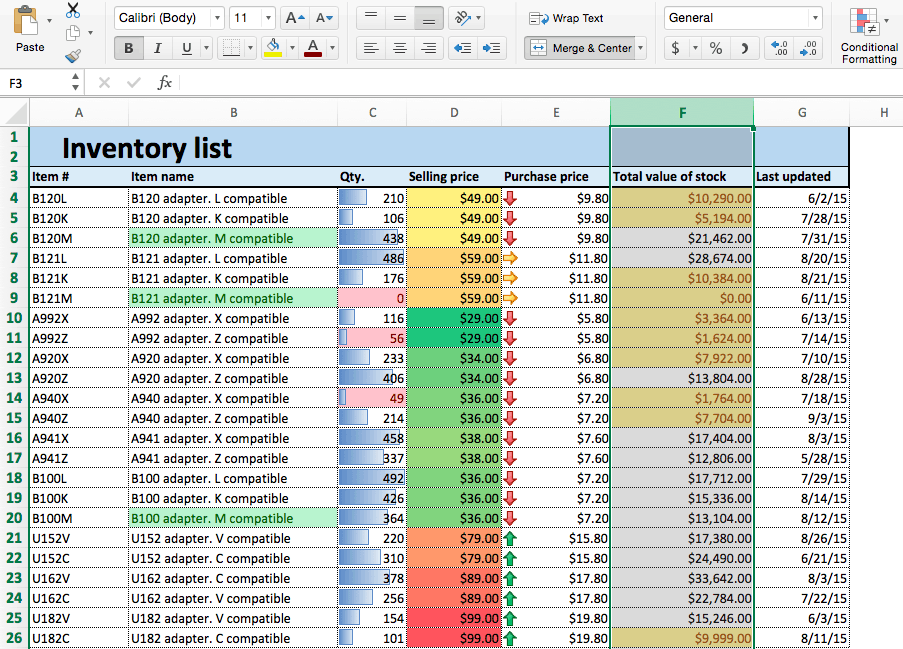
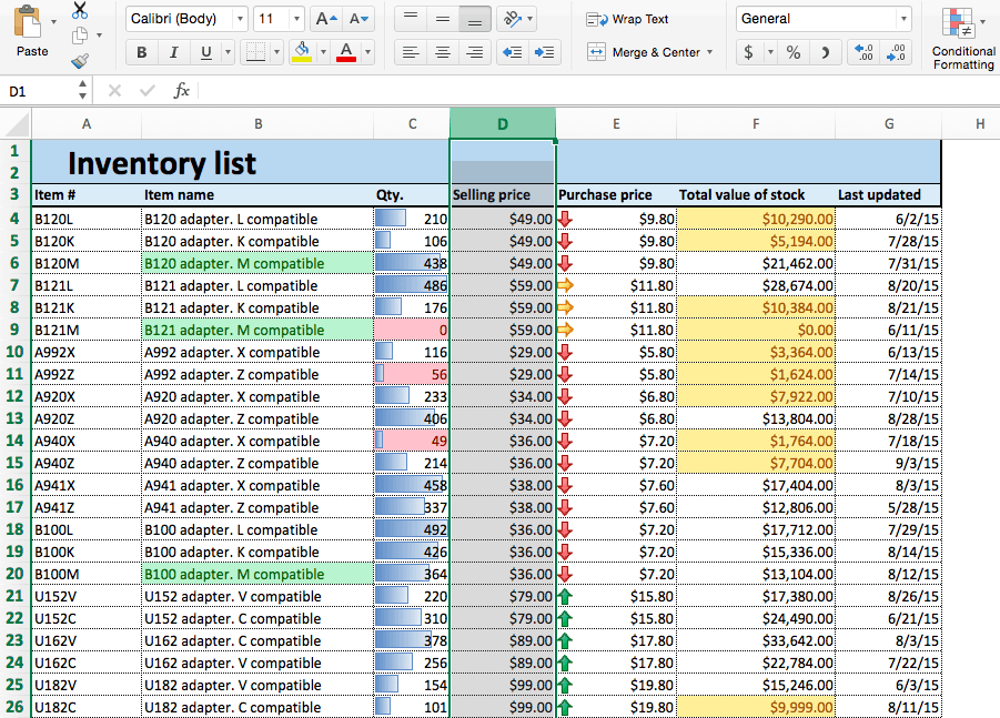
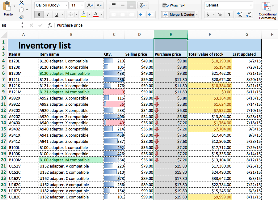
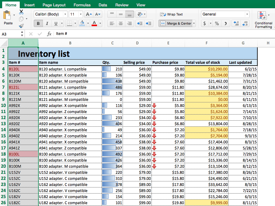
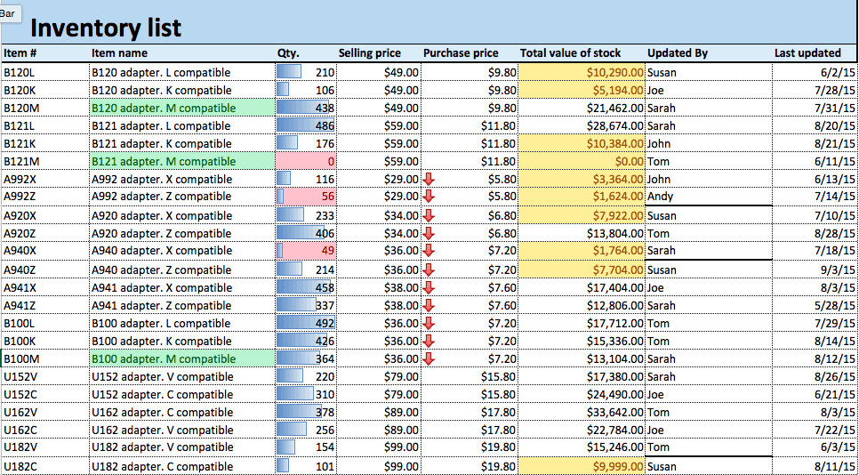
- Open an existing spreadsheet in Excel, or start from scratch and manually enter new data. In this example, we’re using an inventory list that tracks the number of each item currently in stock, as well as some additional information about each product.
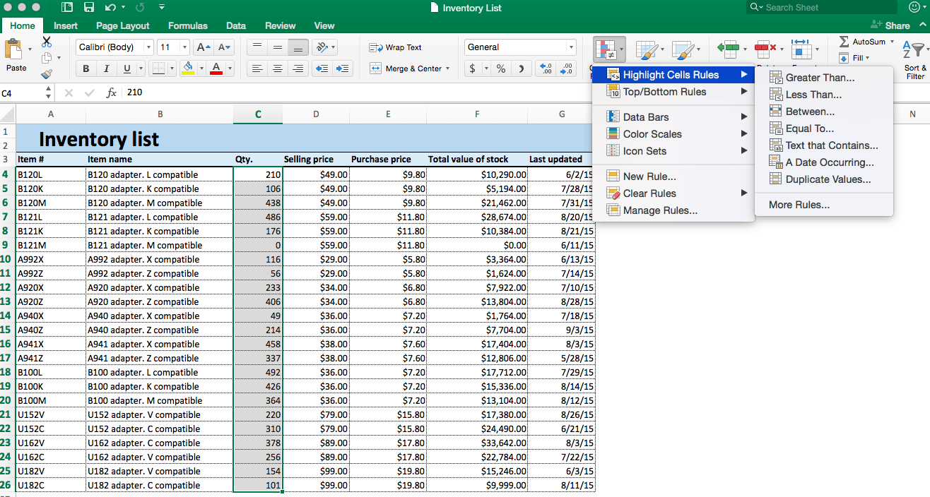
- To apply highlight rules, select the range of values you want to apply a rule to. For this example, we want to highlight any product that’s quantity is less than 100 units. So, select the values in the Qty. column (C4:C26).
- From the Home tab, click Conditional Formatting on the right side of the toolbar, and click Highlight Cells Rules from the dropdown menu. Click Less than.
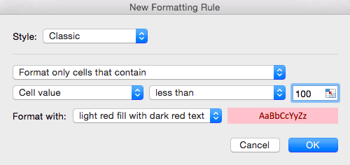
- A box will appear. Type 100 in the empty field. Click OK.
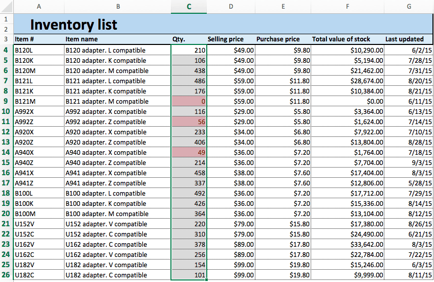
- Your spreadsheet will now reflect this highlight rule, with the quantities less than 100 highlighted red with red text.
Tip: You can change the color of the highlighted cell by clicking on the Format with: dropdown menu and selecting on another option.
- To highlight text cells, repeat step 2. This time, we want to highlight certain model types (M compatible), so we’ll select the cells in the Item name column.
- Click Conditional Formatting > Highlight Cells Rules > Text that Contains…

- Type M compatible in the text box. To differentiate from our previous highlight rule, select green fill with dark green text from the Format with: dropdown menu. Click OK.
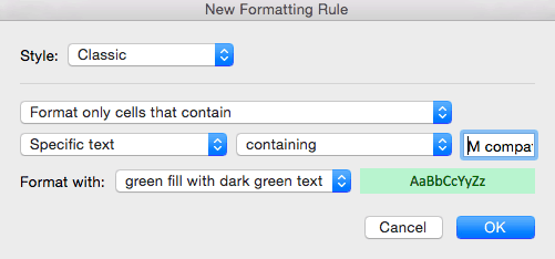
- Now, cells containing the text M compatible are highlighted.
Using these same steps and menu options, you can apply highlight rules to find Duplicate Values, Dates, or values that are Greater than…, Equal to…, or Between… values that you select. All of these possibilities are available through the menu options.
Step 2: Create Top/Bottom Rules
Top/Bottom rules are another useful preset in Excel. These rules allow you to call attention to the top or bottom range of cells, which you can specify by number, percentage, or average.
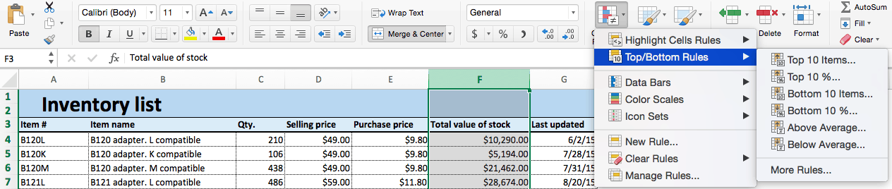
- In this example, we’ll highlight the bottom five total stock values. Click the top of the Total value of stock column to select these cells.
- Click Conditional Formatting > Top/Bottom Rules > Bottom 10 Items… (The default number and percent in Top/Bottom rules in Excel is 10, but you can change that number in the New Formatting Rule box.)
- In the box that appears, change 10 to 5, since we only want the bottom five values. Since we already have a red fill highlight rule, click the dropdown menu and select yellow fill with dark yellow text. Click OK.
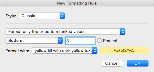
- Your sheet will now highlight the bottom five values in the Total value of stock column, and update as you add to your data set.
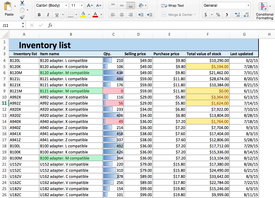
Step 3: Apply Data Bars
Data bars apply a visual bar within each cell. The length of the bar relates the value of the cell to other cell values in the selected range.
- We’ll apply data bars to the Qty. column so we can easily assess the ratios of items in stock. Click the top of the Qty. column to select this range of cells.
- Click Conditional Formatting > Data Bars. You’ll see two options - one for Gradient Fill and one for Solid Fill. They function identically; just select the option and color you prefer.
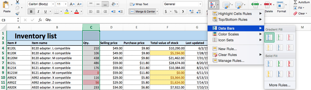
- Your sheet will now reflect the added rule.
Step 4: Apply Color Scales
Color scales are similar to data bars in that they relate a cell’s values in a selected range. However, instead of representing this relationship by the length of a bar, color scales do so with color gradients. One color is assigned the “lowest” value and another the “highest,” with a range of colors in between.
- We’ll apply color scales to our Selling price column. Click the top of column D to select this range.
- Click Conditional Formatting > Color Scales. You’ll see a variety of different color ranges; select the one you want.
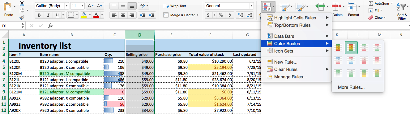
- Your spreadsheet now shows the selling prices by color - red cells are the most expensive, and green cells are the least expensive.
Step 5: Apply Icon Sets
Icon sets apply colorful icons to data. They are simply another way to call attention to important data, and relate cells to one another.
- We’ll apply icon sets to the Purchase price column to show low, middle, and high priced items. Click the top of the Purchase price column to select the range of values.
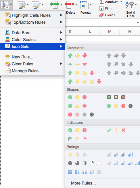
- Click Conditional Formatting > Icon Sets. You’ll see a variety of options for Directional, Shapes, Indicators, and Ratings icons. You can choose any of these to fit the needs of your data. In this example, we’ll choose the first Directional option: red, yellow, and green arrows that indicate high, middle, or low priced items.
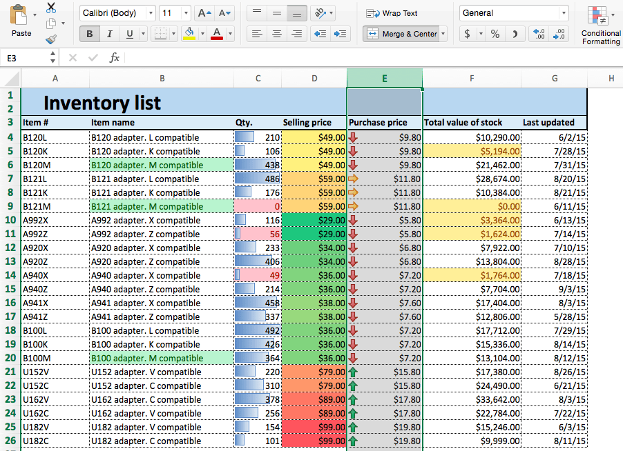
- Your sheet reflects this new formatting rule.
Step 6: Edit and Delete Conditional Formatting Rules
Now you’ve learned the most common conditional formatting presets in Excel, your spreadsheet provides a lot of information at a glance. However, you might want to edit some of these rules later on, or delete them completely.
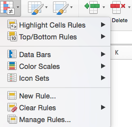
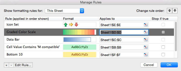
- Click Conditional Formatting and select Manage Rules… from the dropdown list.
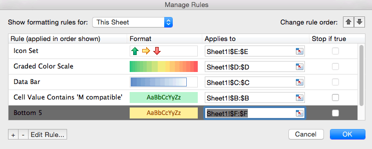
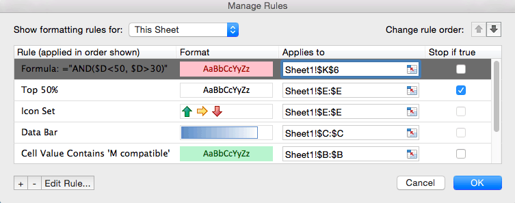
- The Manage Rules box will appear. Click the dropdown menu at the top of the box and click This Sheet to list the conditional formatting rules you have applied to the current sheet.
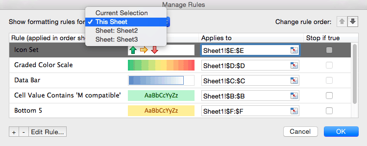
- To edit a rule, click the rule you want to change. In this example, we want to highlight the bottom ten values in the Total value of stock column, rather than the bottom five that we currently have highlighted. Click the Bottom 5 row. Then, click Edit Rule… at the bottom of the box.
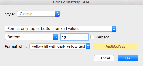
- A new box opens where you can adjust the conditions of the rule. Type 10 in the number field and click OK.
- Excel will bring you back to the Manage Rules box. You must click OK to save the changes you made to the original rule.
- To delete a rule, return to the Manage Rules box and choose This Sheet. Click the rule you want to delete - in this case, the color grading on Selling price. Click the - symbol (next to Edit Rule…) in the lower left hand corner. Click OK.
- The conditional formatting on the Selling price column is now deleted.
You now have everything need to create basic conditional formatting using presets in Excel 2016. For more advanced functionality such as creating a new rule, using Excel formulas, and creating rules dependent on another cell, see the “Advanced” section below.
First, we’ll look at how we can apply the same conditional formatting rules we learned in Excel to another spreadsheet program, Smartsheet.
How to Apply Basic Conditional Formatting in Smartsheet
Use conditional formatting in Smartsheet to apply many of the same rules and effects available in Excel. We’ll guide you through every function described in the previous section, with some modifications that better align with Smartsheet features.
You can create spreadsheets in Smartsheet two ways: by manually entering data into Smartsheet, or by importing an existing spreadsheet from programs like Excel and MS Project. For this tutorial, we’ll use the same data set from the Excel tutorial, so we’ll import the original version (with no conditional formatting) from Excel.
Step 1: Open Your Existing Excel Spreadsheet in Smartsheet
- From the Home screen in Smartsheet, click the + icon. Then, select Import under the Solution Center section.
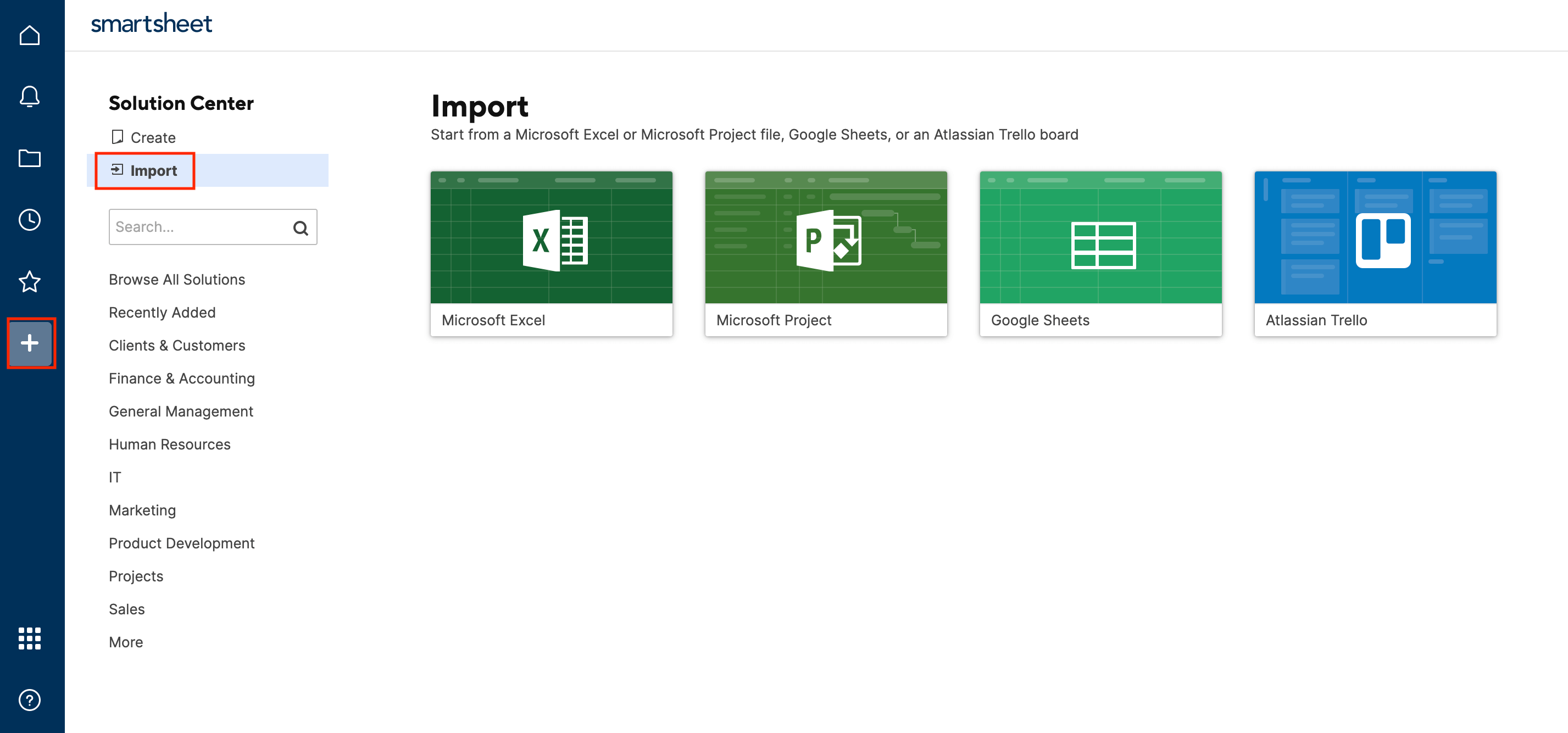
- Click on Microsoft Excel and select the file you want to import.
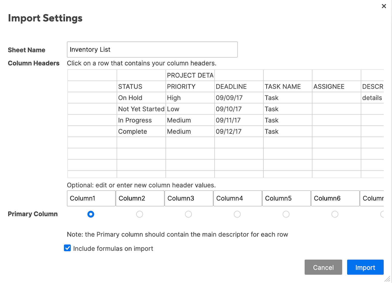
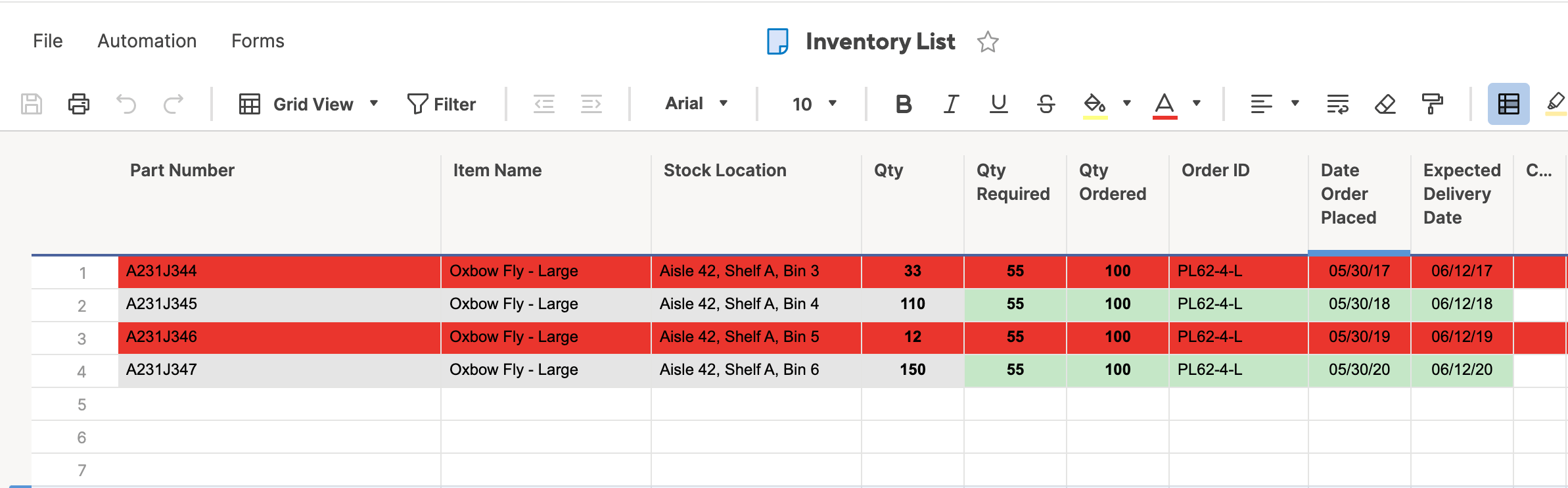
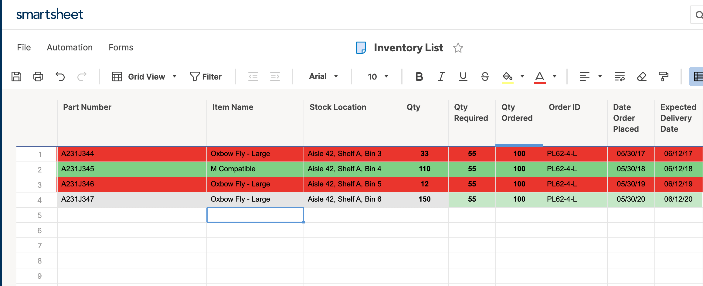
- Name your spreadsheet. We’ll call this one Inventory List. Click Import.
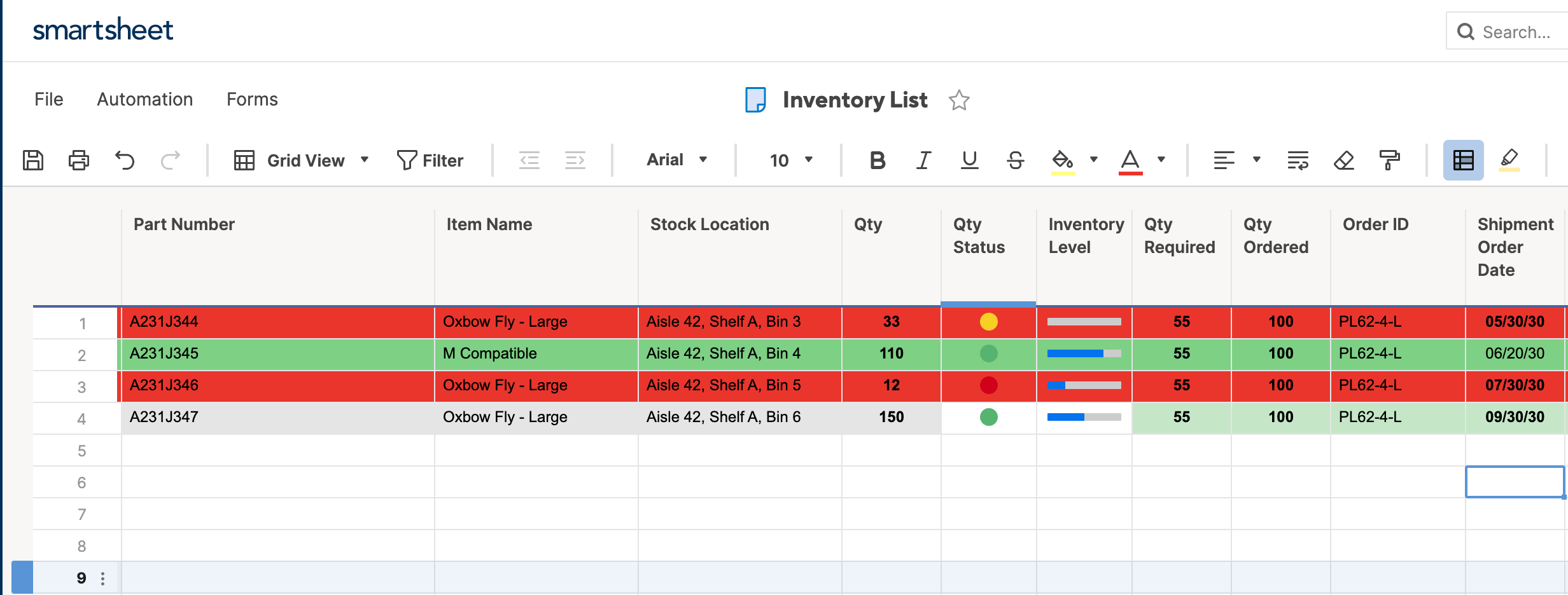
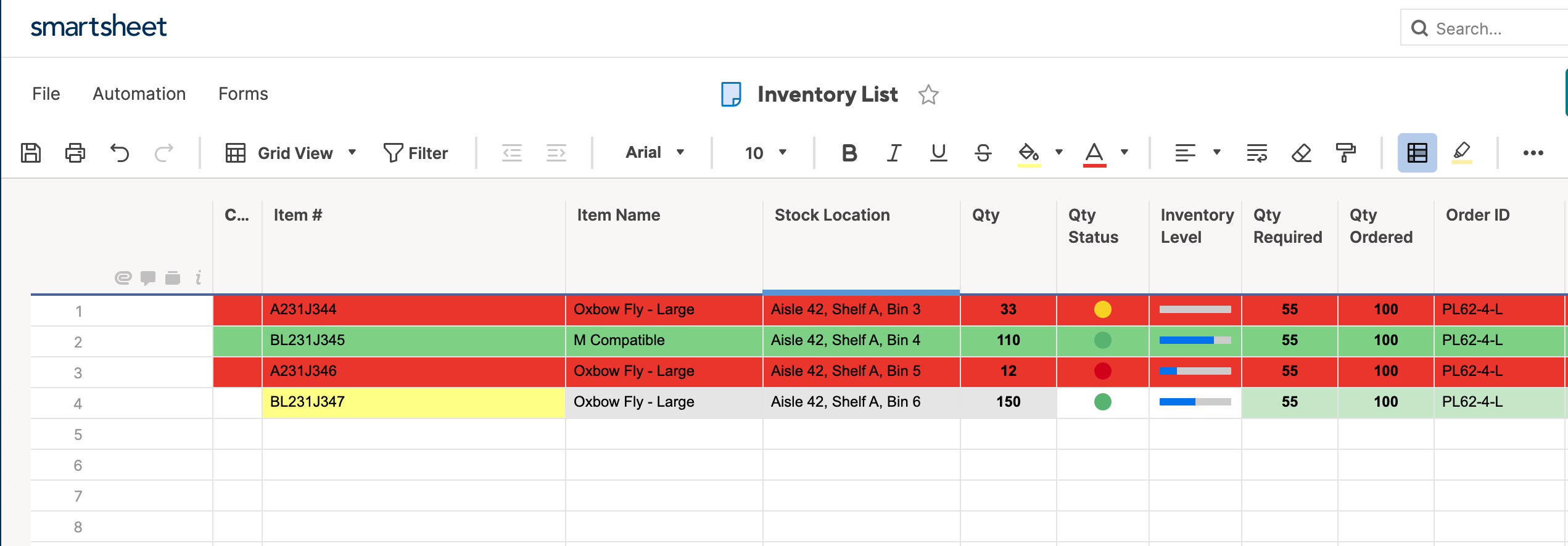
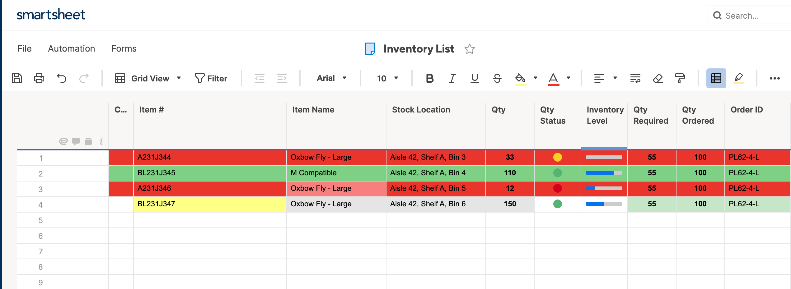
- Your spreadsheet will open, using the same column and row formatting that was applied in Excel. All conditional formatting is controlled through the conditional formatting icon in the toolbar at the top of the app.
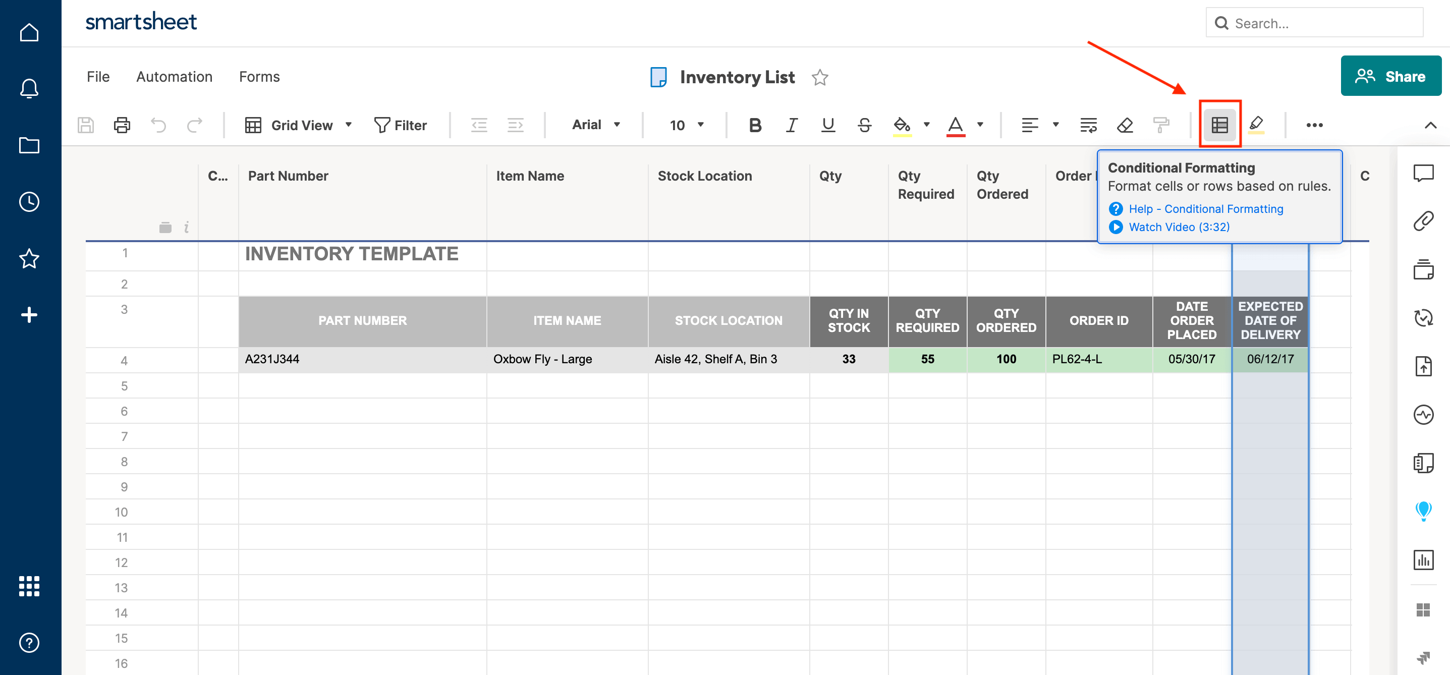
Step 2: Apply Highlight Rules
- To highlight a cell, click the conditional formatting icon on the toolbar.
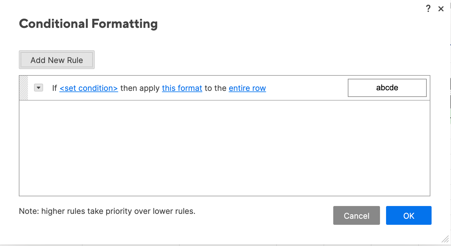
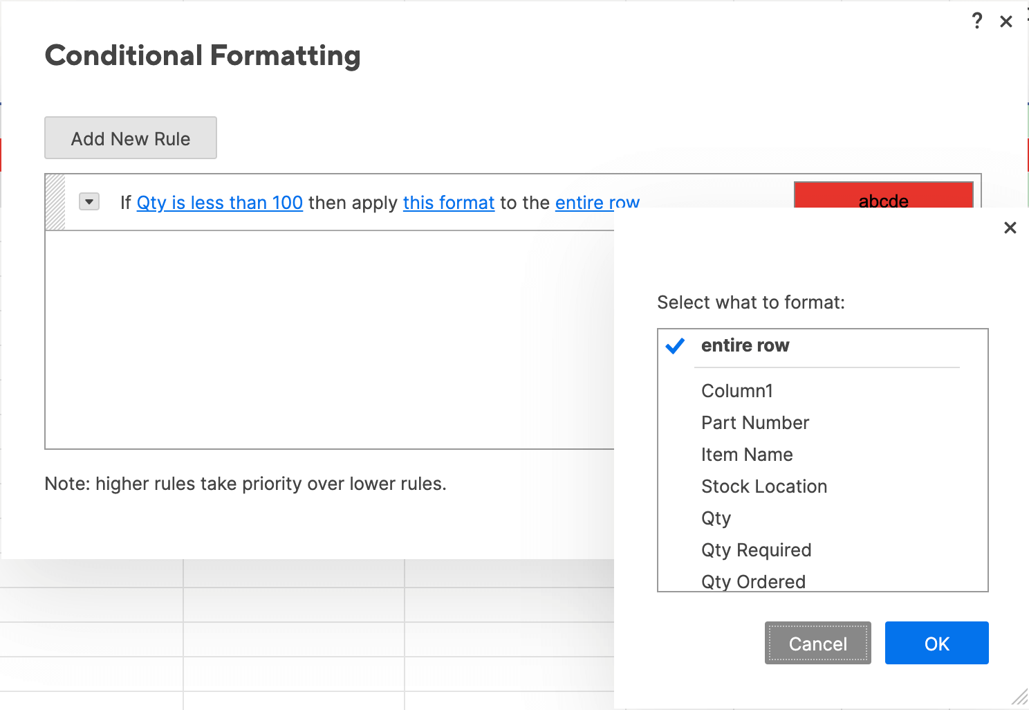
- A box will appear where you can set conditional formatting rules. Click Add New Rule in the top left corner. The if-then logic is already written into the new rule, so you can simply create the conditions.
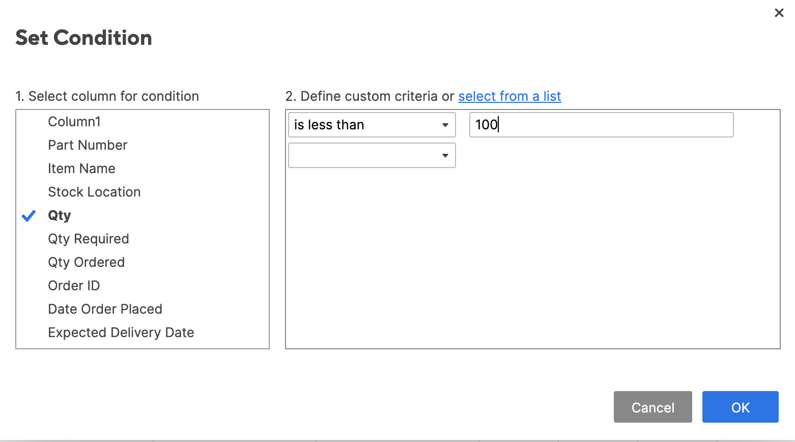
- Click set condition. Just like in the Excel example, we want to highlight any items that are stocked below 100 units. Select Qty. from the column list on the left, select is less than from the center dropdown list, and then type 100 in the field on the right. Click OK.
- Now we need to apply the formatting. Click this format and a dropdown menu with formatting options appears. For this example, we’ll use a paint fill. Click the paint bucket icon and select red.
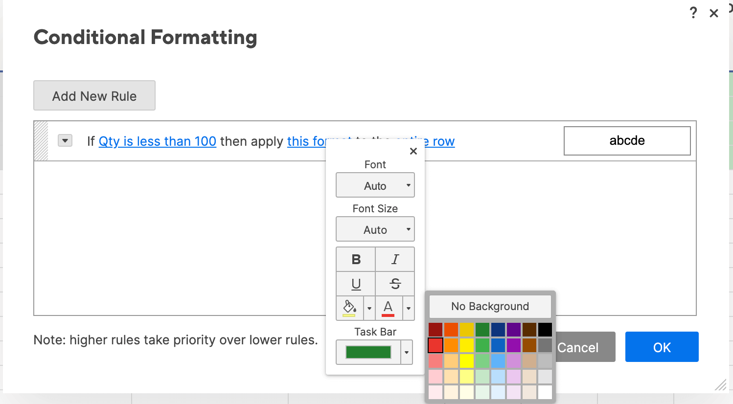
- Specify which cells should get this formatting. Smartsheet will default to format the entire row, but we only want to highlight the cells in the Qty. column. Click entire row and click Qty. from the dropdown list. Click OK.
- Your conditional formatting rule is now reflected in your spreadsheet.
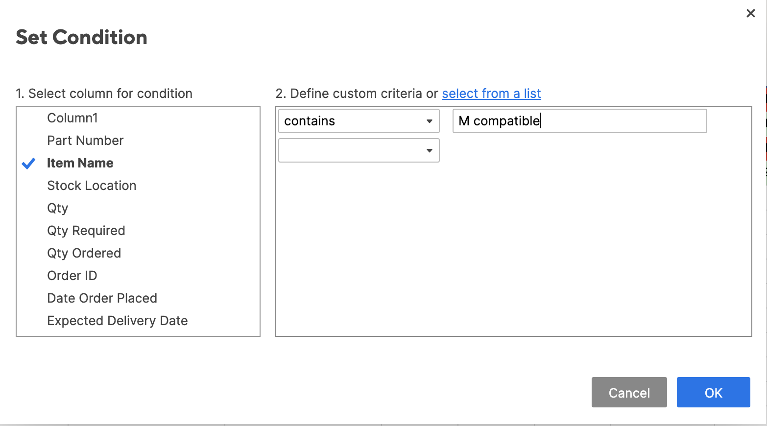
- To highlight text cells, repeat steps 1 and 2. Click set condition. Now, we want to highlight any M compatible items. Select Item name from the left-most list, contains from the center list, and type M compatible in the right field. Click OK.
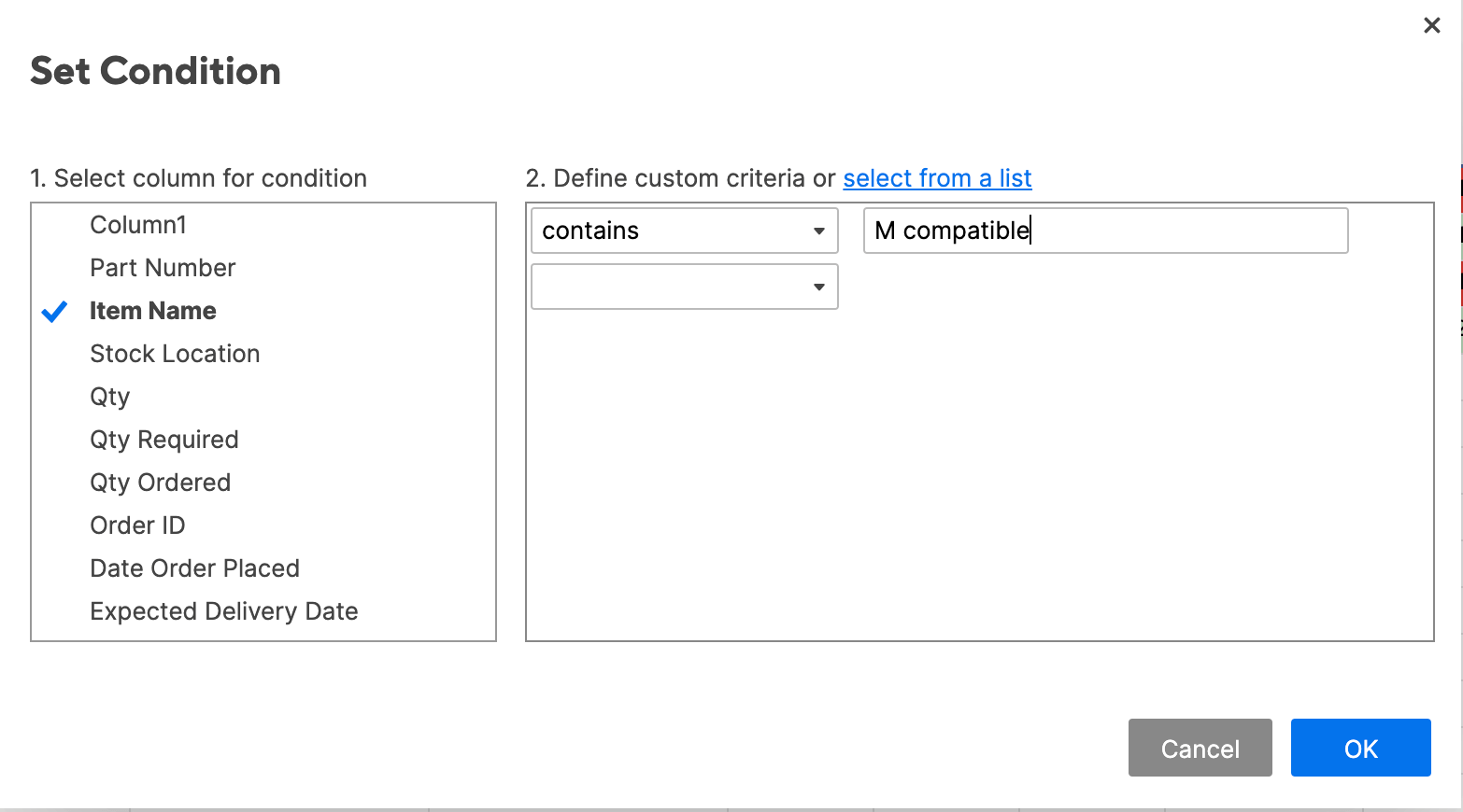
- Click this format and click the paint bucket item. Select green. For this rule, we want to highlight the entire row. (Again, Smartsheet defaults to this option.) Click OK.
- Your second rule is now reflected in your data set.
Step 3: Apply Progress Bars (Data Bars)
In place of Excel’s Data Bars preset, you can create Progress Bars in Smartsheet. Progress Bars are a symbol that you can apply to cells to show and compare the level of completeness. In this example, we’ll apply progress bars to denote current inventory levels (from zero to 100 percent).
- To create Progress Bars in Smartsheet, you first need to create a new Symbols column. Cells in a Symbols column will only hold special characters, such as progress bars.
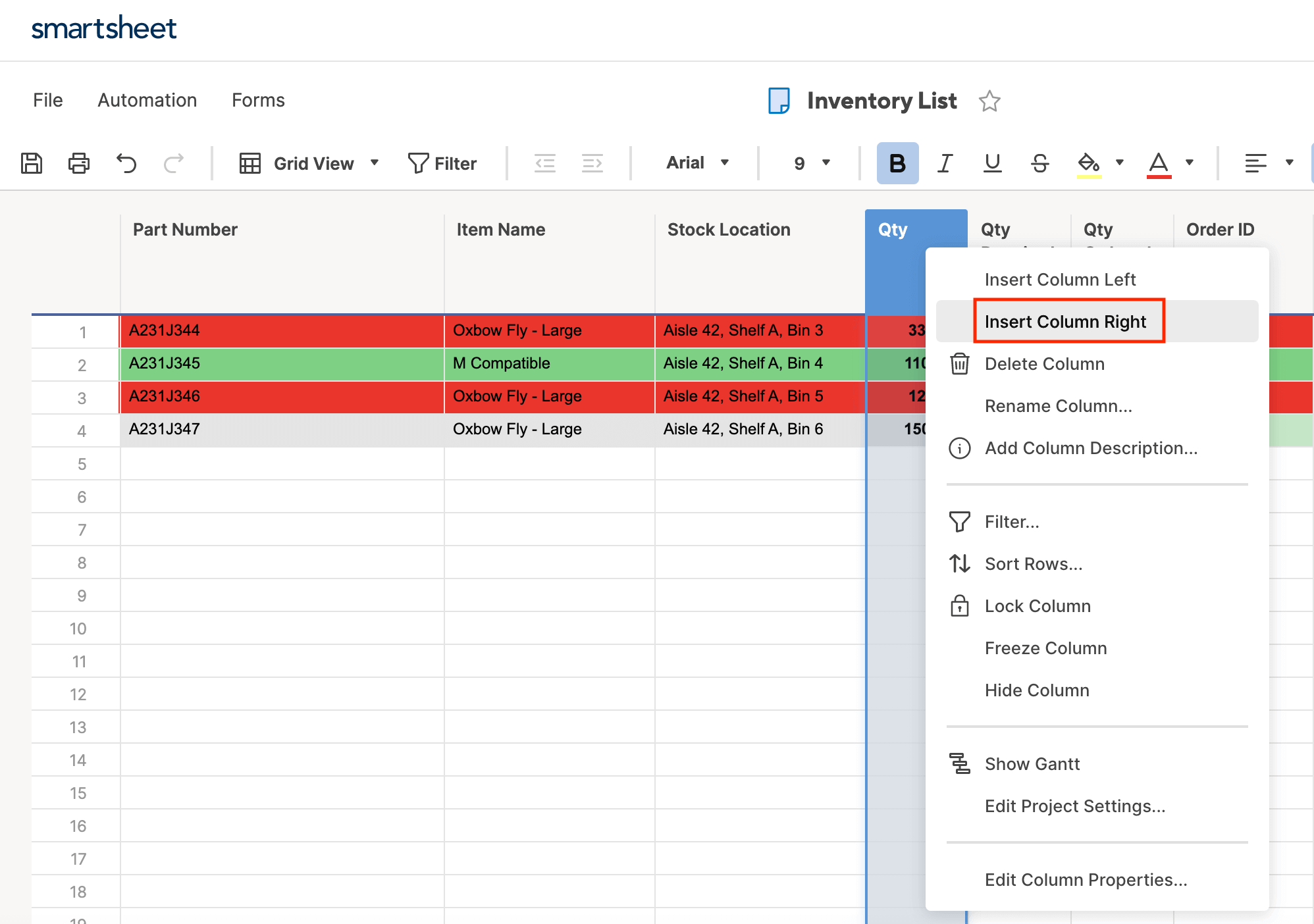
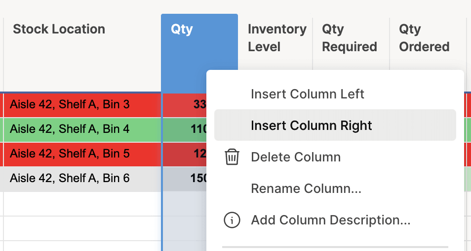
- To create a new column, right-click the Qty. column and click Insert Column Right.
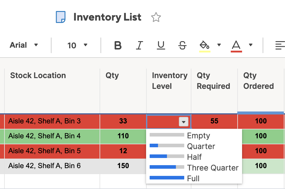
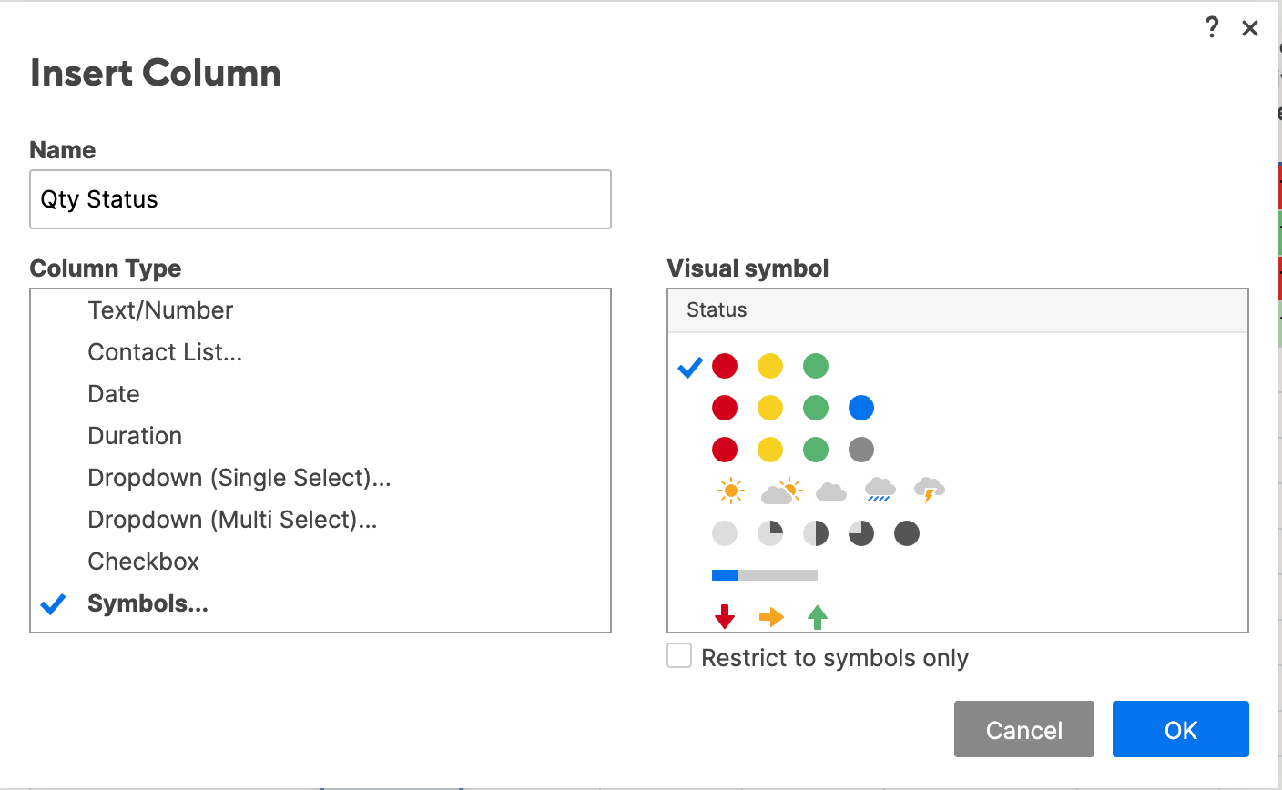
- A box will open. We’ll name this column Inventory Level, and select Symbols... from the list of column-types. In the right-hand field, scroll down and select the progress bar icon. Click OK.

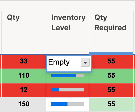
- Click into cells in the new Inventory Level column and select the appropriate level of inventory: Empty, Quarter, Half, Three Quarter, or Full. This progress bar relates the current level (from the Qty. column) to level you need.
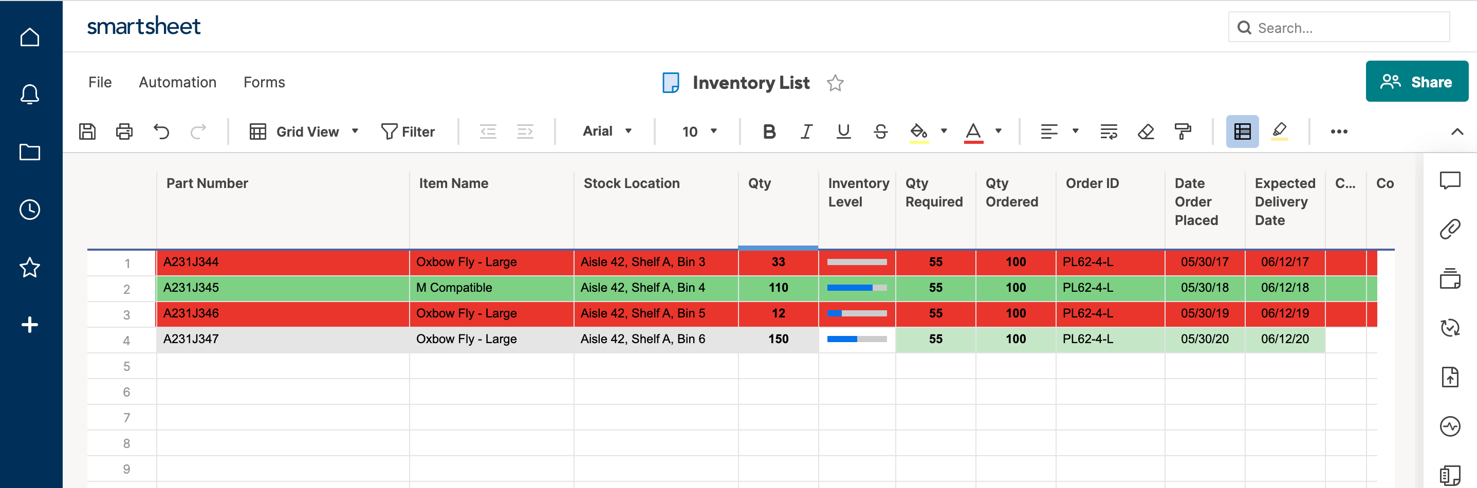
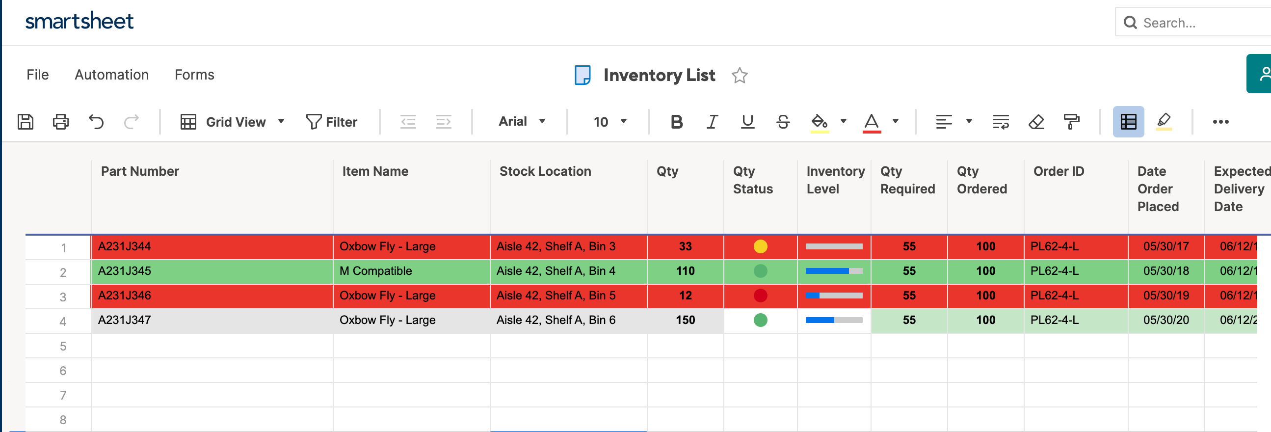
- Here’s what your sheet will look like when all progress bars are filled in.
Tip: You can also type Empty, Quarter, Half, Three Quarter, or Full into each cell, and Smartsheet will autofill with the appropriate progress bar.
Tip: You can also automate progress bars by using an if-then formula in Smartsheet. For more information on how to do this, check out this resource on symbol formulas.
Step 4: Apply Icon Sets
To apply icon sets in Smartsheet with conditional formatting, you’ll have to use formulas (we’ll get into that in the “Advanced” section). Instead, you can add informative icons to your data by creating a special Symbols column.
- Right-click the Qty. column and click Insert Column Right.
- In the box that opens, type Qty. Status in the name field. Click Symbols from the dropdown menu and choose from the library of available symbols (Flag, Priority, Decision, Status, Direction, and Measure icons). In this example, we’ll choose RYG balls in the Status section. Click OK.
- Now, you can update your sheet with the appropriate color status ball by adding conditional formatting as shown above.
Step 5: Edit and Delete Conditional Formatting Rules
Editing and deleting conditional formatting rules in Smartsheet is extremely easy.
- To edit a rule, click the Conditional Formatting icon on the toolbar to open the list of rules. Click the condition you wish to change and edit the information in the box that opens. Click OK.
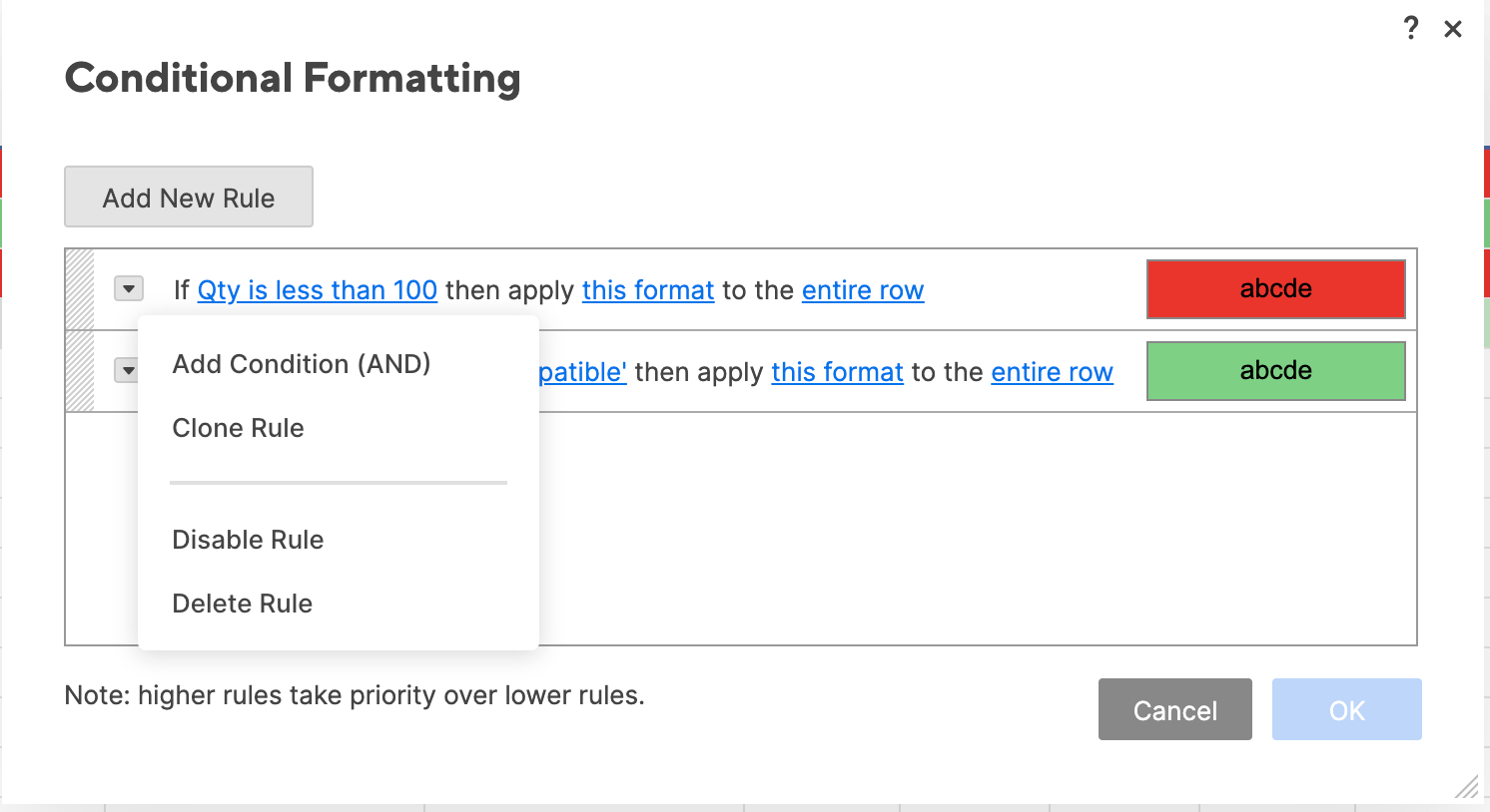
- To delete a rule, click the carrot on the left side of each rule. Click Delete Rule from the dropdown menu. Click OK.
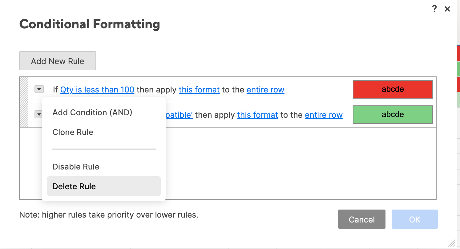
Tip: You can also disable a rule by clicking Disable Rule from the dropdown menu and then clicking OK. This will put the rule on “hold” without deleting it, in case you want to re-enable it later on.
Now you know how to use conditional formatting and other colors and symbols to add formatting to your sheet in Smartsheet. In the following sections, we’ll walk you through more advanced conditional formatting functions in Excel and Smartsheet.
Advanced Conditional Formatting Functions in Excel
Once you have mastered the basics, Excel includes some additional advanced conditional formatting functions. We’ll guide you through applying stop-if-true rules, using the AND formula, setting rule hierarchies and precedence, and other unique situational formatting conditions below.
Step 1: Create a New Rule and Apply Stop if true Rule
In some instances, you might want to stop a certain condition, without deleting the entire rule. The Stop if true rule in Excel enables you to do so.
- In our example, we applied an icon set of three directional arrows to the Purchase price column to indicate low, medium, and high price ranges. However, we might actually only want to call attention to the lowest cost items, as three icons can clutter the sheet (and provide more information than actually needed).
- First, create a separate condition on this column. Click the Purchase price column to select these values.
- Click Conditional Formatting > Manage Rules… to open the Manage Rules box. Keep the default Show formatting rules for: Current Selection from the dropdown menu, because we are only adjusting the rule on this column.
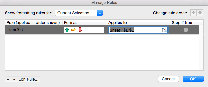
- Click the + in the bottom left corner to create a new rule. A new box opens where you can assign conditions to the new rule.
- From the Style menu, select Classic.
- Instead of applying a different icon to bottom, middle, and top price ranges (as we currently have), we only want to show the bottom 50 percent. So, select Top from the left dropdown menu, type 50 in the middle field, and check the Percent box.
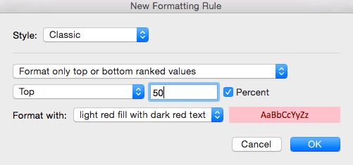
- To apply color formatting, Select Custom format from the Format with dropdown menu, and a new formatting box opens. Click the Fill tab, and click No Color.
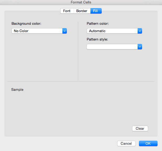
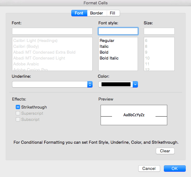
- Next, click the Font tab, and select black text. Click OK.
- Click OK again in the original New Formatting Rule box.
- You’ll return to the Manage Rules box, where you now have two rules applied to the Purchase price column. Click the Stop if true box to the right of the new rule you just created. Click OK.
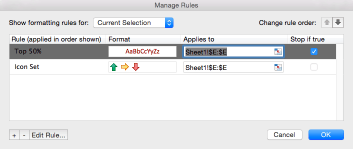
- Your sheet will now only show the icon sets for the items with a purchase price in the bottom 50 percent.
Step 2: Apply Multiple Conditions to a Rule with AND Formula
Adding Excel’s formulas to your conditional formatting rules is one way to elevate your logical rules. The AND formula is one of the most popular, easy-to-use formulas. It lets you add multiple conditions within a single rule, rather than writing out each rule separately. To format cells they must meet both conditions.
- We’ll create a new rule to highlight any cell in the Item # column that contains both a B and an L. Click the top of the Item # column to select this range of cells.
- Click Conditional Formatting > New Rule.
- In the dialogue box, select Classic from the top dropdown list. Select Use a formula to determine which cells to format, since we’re using a formula.
- We want to search cells in the Item # column for a B and L, and highlight that cell when both conditions are true. To do this, we’ll use Excel’s ISNUMBER and SEARCH formulas, with the AND formula, to look for the B and L values.
- =AND(ISNUMBER(SEARCH("B",A1)),ISNUMBER(SEARCH("L",A1)))
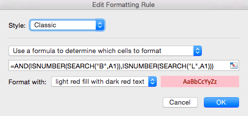
- Click OK. Your sheet will highlight all cells in Item # that meet both of these conditions.
Tip: Understanding the formula:
- We use AND at the beginning of the formula to show that both of the following conditions must be met in order to apply the conditional formatting.
- The basic syntax of the nested formula is ISNUMBER(SEARCH(“substring”,text)) where “substring” is the character(s) you are looking for, and “text” is the cell(s) you want to search.
- We are searching for two separate conditions, so we write the ISNUMBER(SEARCH(“substring”,text)) formula twice, separated by a comma.
This example is just one of hundreds of different formulas you could enter with the AND function. For more information on using Excel formulas with conditional formatting, click here.
Step 3: Conditional Formatting Based on Another Cell
You can also create rules to highlight certain cells based on the value of another cell.
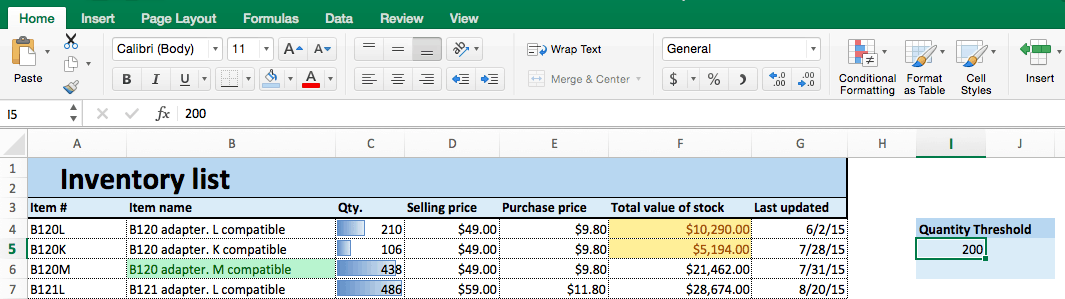
- In this example, we’ll create a “quantity threshold” - items with inventory level below this threshold will be considered “at risk.” We already have a rule that highlights cells in the Qty. column under 100. However, that threshold might change over time, depending on manufacturing or selling rates. So, we want to create a highlight rule that is dependent upon a threshold that we set.
- To the right of your data, create a box for Quantity Threshold and choose an amount. In this example, we use 200. (Note the cell you type the amount in. Here, it’s I5.)
- Create a new rule by clicking Conditional Formatting > New Rule.
- In the dialogue box, click Classic and Use a formula to determine which cells to format from the dropdown menus.
- In the formula field, type =C4<$I$5 and keep the default formatting. Click OK.
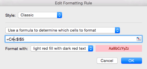
- Numbers in the Qty. column that are less than the Quantity Threshold in I5 (200) will now be highlighted.
- Now, you’ve created a dynamic rule. This means that as your threshold changes, the rule will still be applied to the Qty. column and the formatting will adjust as appropriate.
Tip: Understanding the formula:
- In this formula, we are simply testing whether or not values in column C are less than the value in I5.
- Start with “=C4” to tell Excel where we want to start evaluating values from.
- Use ‘$’ symbol around I because it’s an absolute value - we are only evaluating cells in column C against this single cell.
Step 4: Data Validation and Dropdown Lists
While data validation is not technically monitored through conditional formatting rules, you can use it to a similar effect: controlling the formatting of your sheet. You can apply data validation to ensure that any cell-type only allows certain entries (text or numbers only, text length, etc.). In this example, we’ll show you how to create a dropdown list and validate data only from that dropdown list.
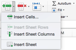
- We’ll create an additional column of which employee last updated the sheet, and create a dropdown list to choose from. First, click where you want to add the column on the sheet. Create a new column by clicking Insert > Insert Sheet Columns from the ribbon on the Home tab.
- We’ll name this column Updated By.
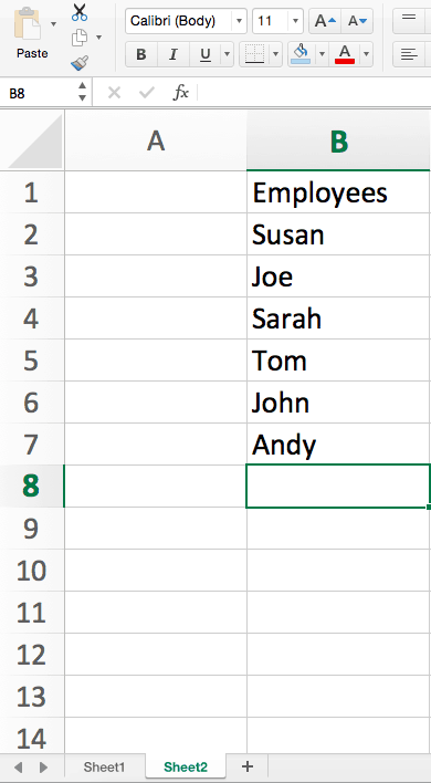
- Now we need to make a list of employees, that the dropdown list will later pull from. Create a second sheet (in the same Excel workbook) by clicking the + sign on the tab at the bottom of the spreadsheet, and write a list of employee names in column B.
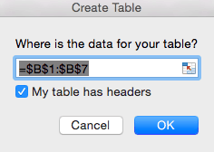
- Select the range of data (all the names) you want to include in your list. Make this list into a table by clicking the Insert tab > Table.
- The dialogue box will show the range of data you selected for the table. Click My table has headers, since we began the list with Employees. Click OK.
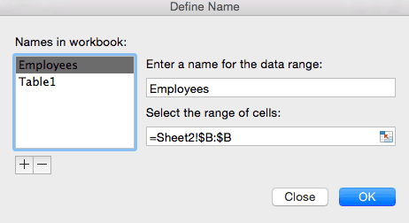
- Now we have to name this list so that Sheet 1 can pull from it. Click Formulas tab > Define Name on the ribbon.
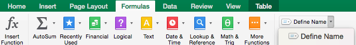
- In the dialogue box, type the name of the list. We’ll call it Employees. Double check that the selected range is still correct. Click OK.
- Go back to Sheet 1. Now, we have to make the Updated By column into a dropdown list. We’ll use the data validation function to do this.
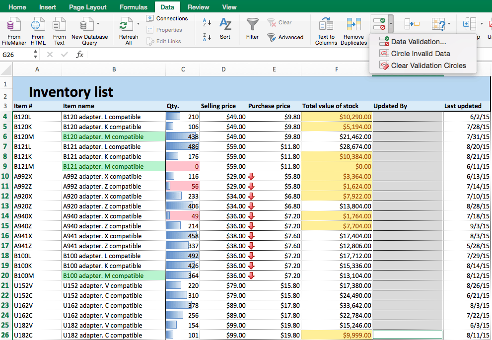
- Select the Updated By column to apply data validation to this range of cells.
- Click the Data tab on the ribbon and click Data Validation > Data Validation…
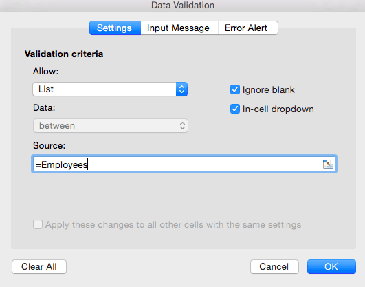
- In the dialogue box, choose List from the dropdown menu to restrict data entered in this range to a list. Type =Employees in the Source field, since we’re pulling from the list we just created (in Sheet 2). Click OK.
- There is now a dropdown list in the Updated By column. Your sheet will only accept data in this column that comes from the Employees list on Sheet 2.
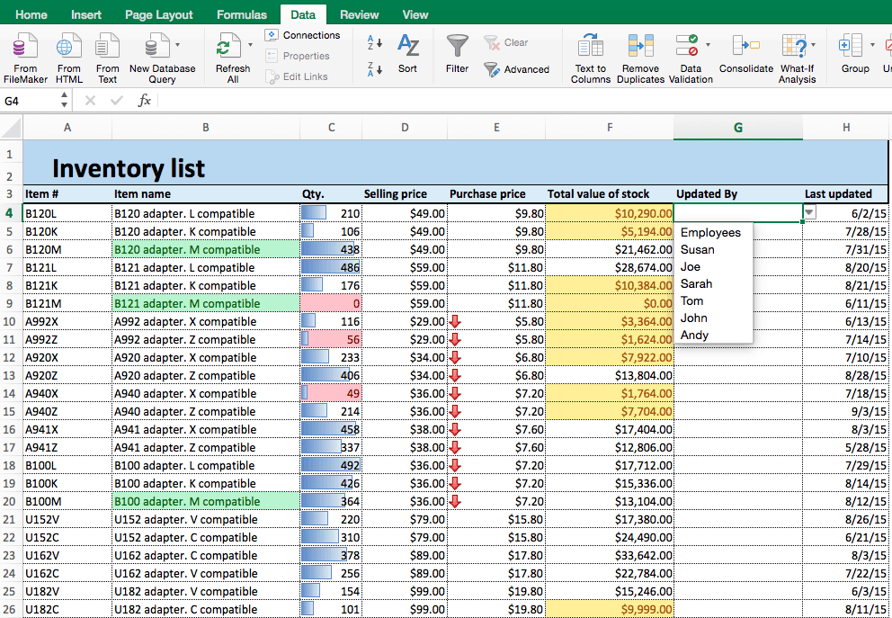
- You can now fill in the column by selecting a name from the dropdown list.
Step 5: Rule Hierarchy and Precedence
As you accumulate conditional formatting rules, watch out for rule hierarchy. Since you can apply multiple conditions to a cell (or row), they occasionally conflict. When this happens, Excel has default precedence rules that may cause one rule to override another, so you can lose your formatting. To combat this, you can change the hierarchy of the rules.
Adjusting rule hierarchy in Excel is straightforward, but you should also understand the logic behind rule precedence:
- Newer rules will always assume precedence over older rules. This means that the precedence of your rules will be in the reverse order of how you created them.
- When multiple rules evaluate as true to a cell, they may or may not conflict. Applying multiple rules to a cell does not necessarily mean that they will interfere.
- Rules don’t conflict if they are changing different things about the cell. For instance, if one rule changes text color and another changes fill color both rules should co-exist in the cell.
- Rules conflict when the outcomes are the same. For instance, if one rule changes a font color to green and another changes the font color to blue the newer rule takes precedence.
To adjust rule hierarchy in Excel, follow these steps:
- All rule hierarchy is controlled through the Rule Manager in Excel.
- From the Home tab, click Conditional Formatting > Manage Rules… to open the Rule Manager.
- Select This Sheet from the top dropdown list to pull up all lists applied to the current sheet.
- To change the order (hierarchy) of rules, select a rule and click the up and down arrows in the top right corner to move it. Click OK. Remember the rule closest to the top will take precedence.
Advanced Conditional Formatting in Smartsheet
Many advanced Excel conditional formatting options are available to Smartsheet users, as well. We’ll teach you how to apply stop-if-true rules, create rules with multiple conditions, create formatting rules based on other cells, and set rule hierarchies and precedence.
Step 1: Add New Rule and Apply Stop If True Function
Adding a new rule in Smartsheet is easy (you already learned how in the “Basic” section). Now, we’ll apply the same “stop if true” logic from Excel in Smartsheet.
- Add a new rule by clicking the conditional formatting icon on the toolbar. Click Add New Rule and click Set condition.
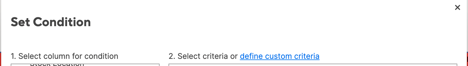
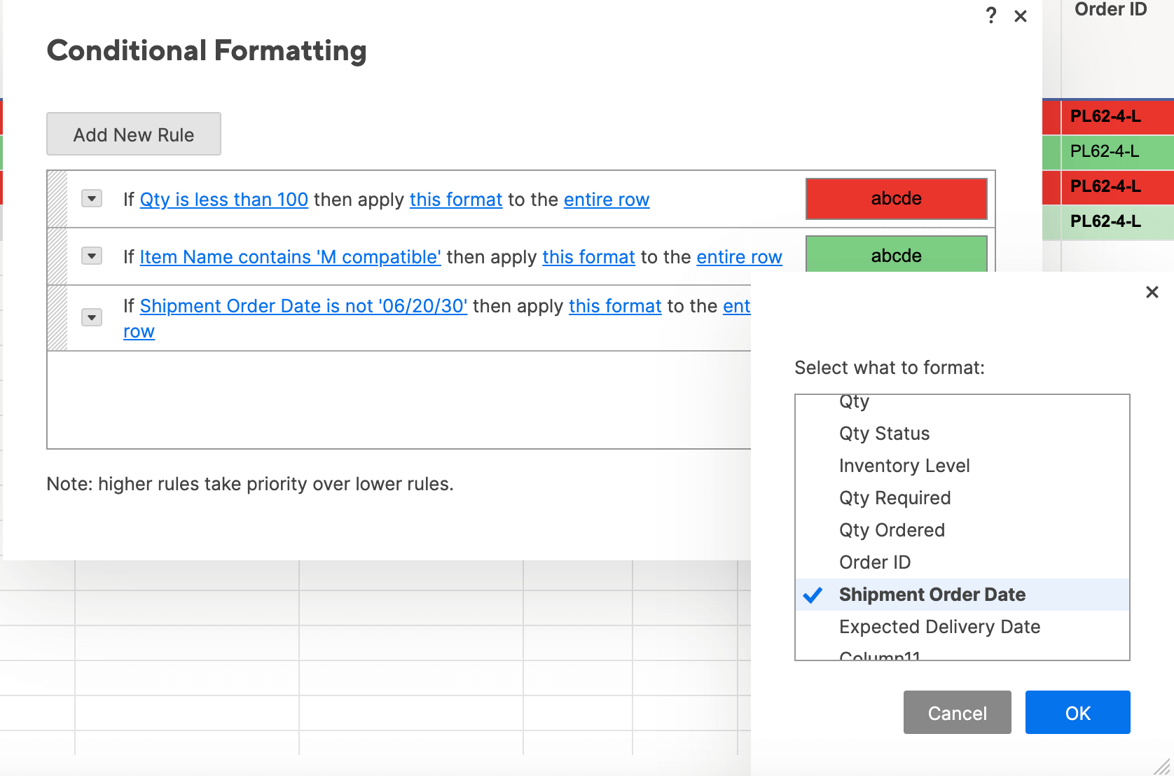
- For this rule, we want to call attention to the shipment order dates that are after 06/20/30. The easiest way to do this is to apply the same logic as “stop if true” in Excel.
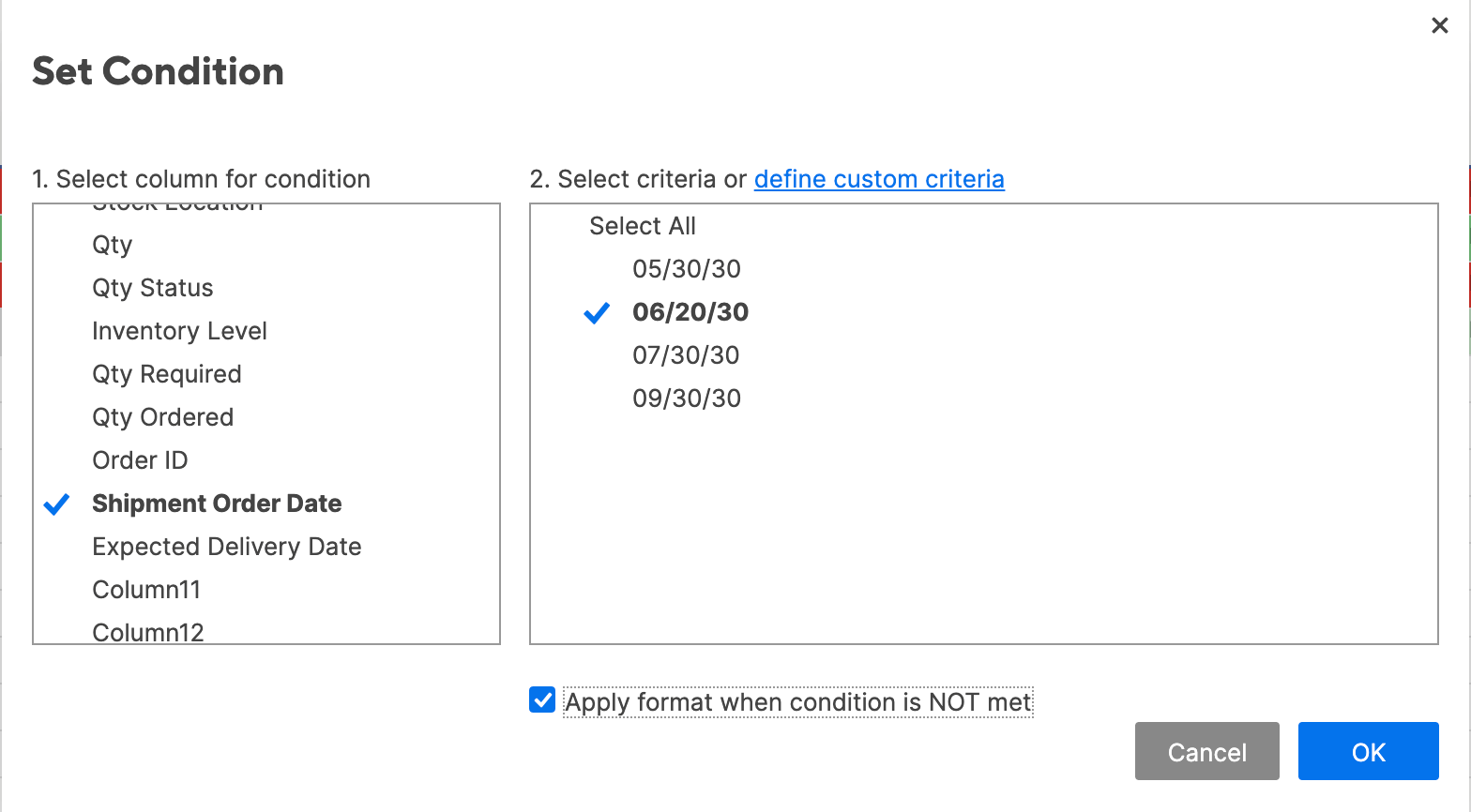
- Click Shipment Order Date in the left field to set a condition in this column.
- Instead of defining criteria (as we have been doing), click select from a list. The list of values in the Shipment Order Date column appear.
- Click 06/20/30. Then, because we want to highlight all the dates that are not this date, check the Apply format when this condition is NOT met box. (This functions just like the “stop if true” box in Excel.) Click OK.
- Click this format and apply whatever format you want. We’ll make the text bold.
- Click entire row and select the Shipment Order Date column. Click OK.
- Now, all dates other than 07/01/15 will be bolded in the Shipment Order Date column.
Step 2: Add Multiple Conditions to a Rule
Just like in Excel, you can use Smartsheet’s built-in formulas when creating conditional formatting rules. However, Smartsheet makes it easy to perform some of the simple functions that basic Excel formulas provide, so you don’t have to worry about remembering complicated formula syntax. To perform the AND function, you can simply click to add multiple conditions to any conditional formatting rule.
- Click the conditional formatting icon on the toolbar and click Add New Rule.
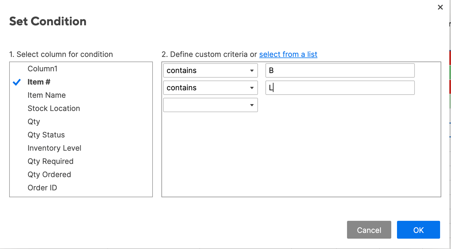
- Click set condition. We want to highlight cells in the Item # list that contain both a ‘B’ and an ‘L.’ Click Item # from the dropdown list on the left.
- For the conditions, select contains and type B. Click into the second prompted condition and type L to create the second condition. (This will perform the AND function.) Click OK.
- Apply the formatting to your rule. We’ll use a yellow fill.
- Change entire row to Item #. Click OK.
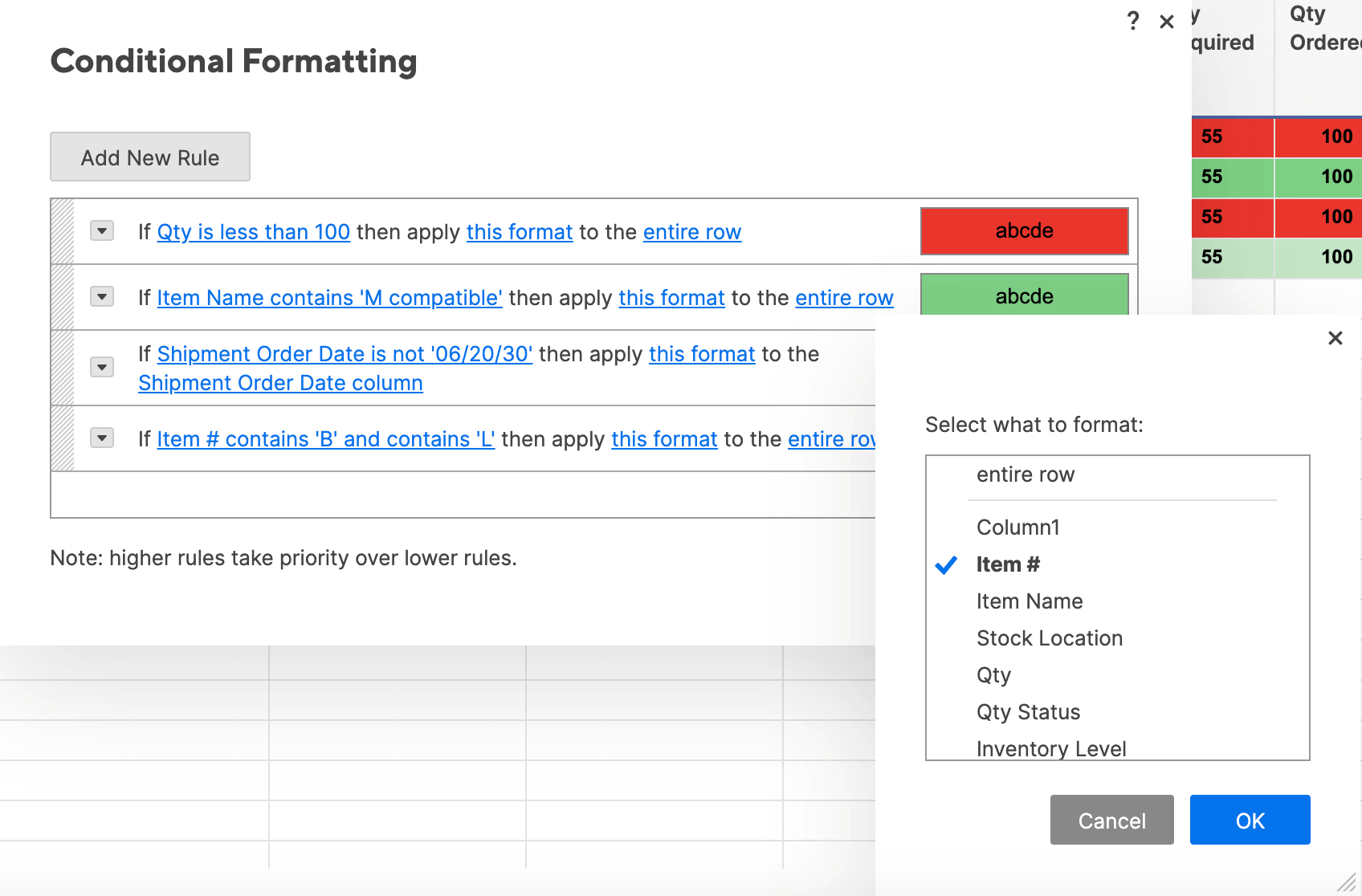
- Your sheet will now highlight those values in Item # that contain both a B and an L.
You can still use formulas with conditional formatting, if you’d like. For an introduction on how to use formulas, check out this resource.
Step 3: Conditional Formatting Based on Another Cell
Smartsheet also makes it easy to apply conditional formatting based on another cell. Instead of using complicated formulas to reference different cells, you can simply control which cells to pull from and format with a few clicks.
- In this example, we want to highlight the Item Name column if the status bar is red, to call attention to at-risk items. To do this, we’ll create a rule that pulls from the Qty. Status column, but applies formatting to the Item Name column.
- Click the conditional formatting icon on the toolbar and click Add New Rule > set condition.
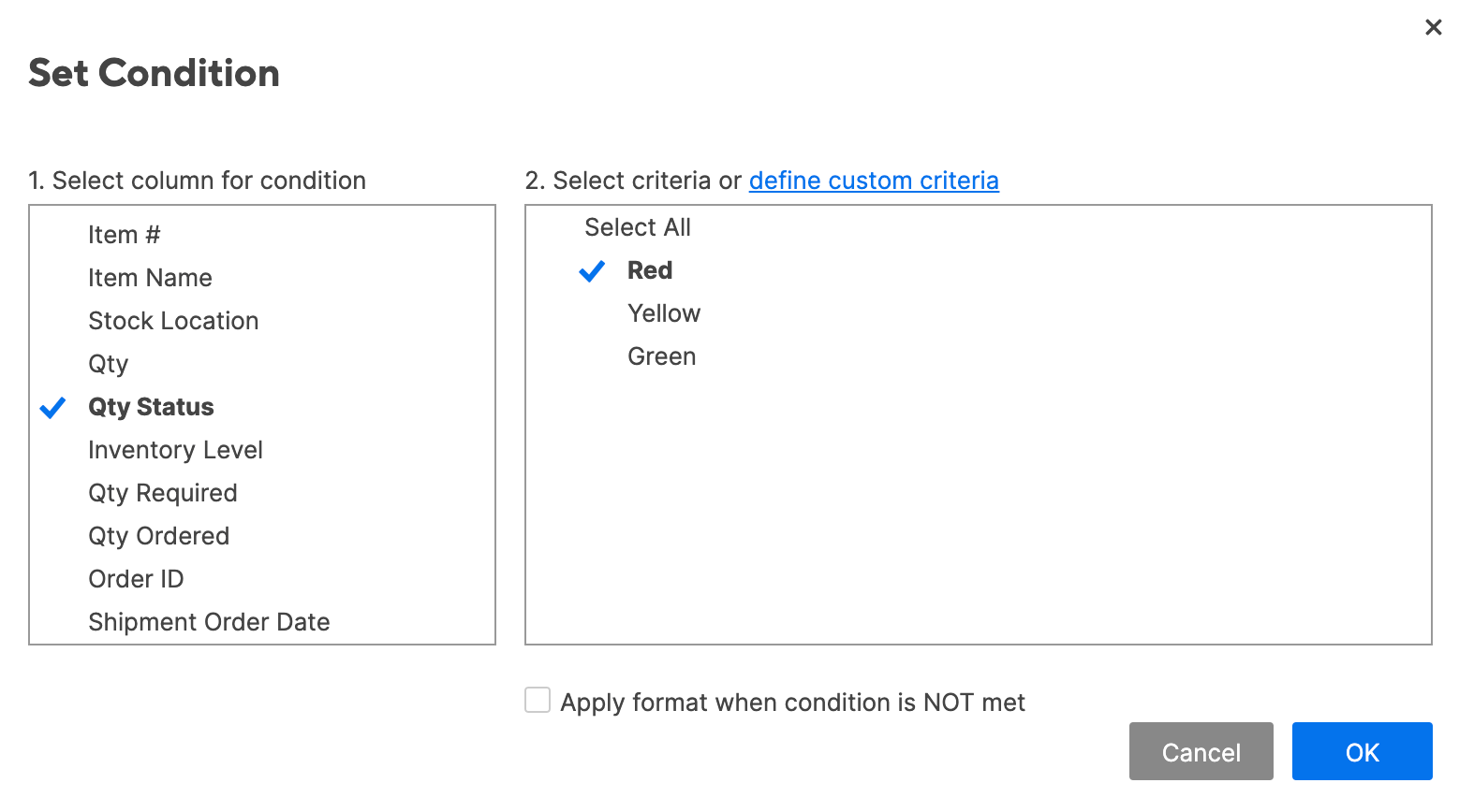
- Click Qty. Status from the drop down list and click Red. Click OK.
- Apply a light red paint fill to format with.
- Click entire row and select Item name. This will apply formatting to cells in the Item name column, even though we’re pulling information from the Qty. Status column.
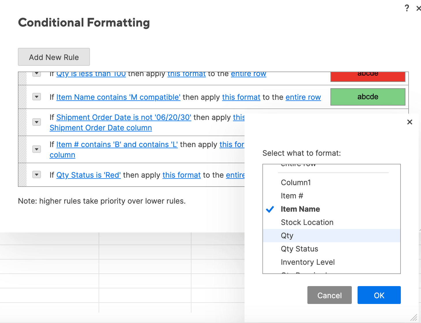
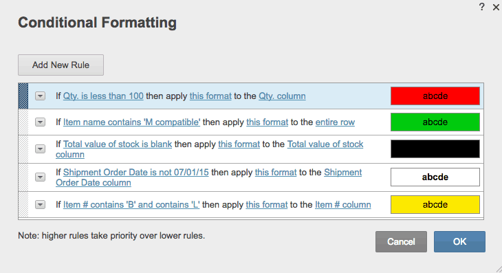
- Click your new rule and drag it to the top of your rules list. Since we have multiple highlighting rules, this will ensure that this rule takes precedence over others.
- Cells in Item Name will now be highlighted if the Qty. Status ball is red.
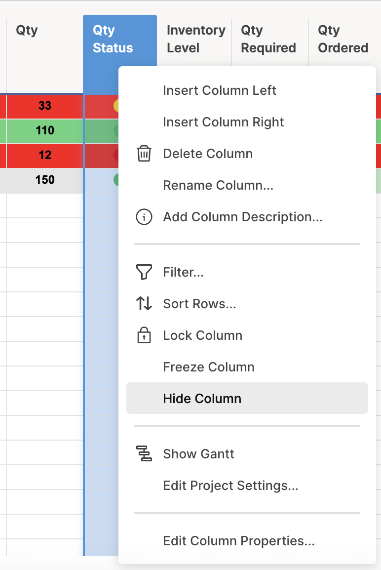
Tip: To eliminate visual redundancy, you can hide the Qty. Status column in your sheet. Simply right-click the column and click Hide column. Your sheet will retain its formatting based on that column, but it will look cleaner.
Step 4: Rule Hierarchy and Precedence
Managing rule hierarchy is quite simple in Smartsheet. The rules also interact the same way as Excel (you can apply multiple rules to a single cell, but only one will show up if there’s a conflict). However, the default precedence is a little different:
- Click on the conditional formatting icon to bring up the rules.
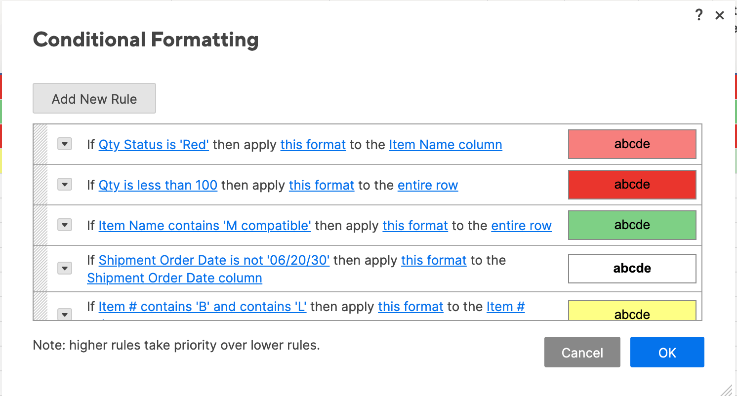
- In Smartsheet, rules higher on this list have precedence. So, the rules have descending hierarchy from the top to bottom of the list.
- To change hierarchy, simply click on a rule and drag it up or down.
Frequently Asked Questions About Conditional Formatting
The most commonly asked questions about conditional formatting include queries about who can make changes, where to learn about using formulas, and how to copy conditional formatting rules between sheets. We’ve answered these and other frequently asked questions below:
Will conditional formatting change the values in my cells?
No. Conditional formatting only applies formatting to your cells. However, you can use conditional formatting to manipulate the values in your cells by using formulas, or by creating rules that change the value of a cell based on another cell.
Can anyone change or apply conditional formatting to the spreadsheets?
Only one person can update conditional formatting rules in Excel at a time. In Smartsheet, any collaborator with Admin permissions can create or edit conditional formatting, but editors and viewers cannot. Click the Sharing button to adjust permissions.
Does the Office 365 (cloud) version of Excel support conditional formatting?
Users can only view conditional formatting in the cloud version of Excel. To add or edit rules, download the Office 365 desktop version. Be careful of version control issues when working with Office 365.
I’m not comfortable using Excel formulas. Where can I learn more?
Here is a list of common questions for using Excel formulas with conditional formatting. For a comprehensive list of all Excel formulas, click here. For help with using formulas with conditional formatting in Smartsheet, check out these tips.
How do I add conditional formatting to a new document in Excel?
To copy conditional formatting to a new workbook or sheet, select the cells you want to copy conditional formatting from, and click the Format Paint icon. Drag your cursor over the column, rows, or document to apply the rules.
Here’s a walkthrough of this function.
Keep Your Team in Sync with Real Time Conditional Formatting in Smartsheet
Empower your people to go above and beyond with a flexible platform designed to match the needs of your team — and adapt as those needs change.
The Smartsheet platform makes it easy to plan, capture, manage, and report on work from anywhere, helping your team be more effective and get more done. Report on key metrics and get real-time visibility into work as it happens with roll-up reports, dashboards, and automated workflows built to keep your team connected and informed.
When teams have clarity into the work getting done, there’s no telling how much more they can accomplish in the same amount of time. Try Smartsheet for free, today.