How to Use VLOOKUP: Step-by-Step Tutorials, Tip Sheets, and More

In an Excel spreadsheet, formulas are helpful because they calculate mathematical, logical, and statistical actions, and you can add these formulas in your spreadsheet to automate data generation. Excel has functions that are preset formulas, or you can enter your own. The Excel function wizard is a special feature in Excel that provides a shortcut to writing formulas. All the possible Excel formulas are in the function wizard, but not the combination of formulas.

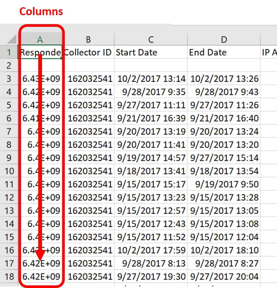
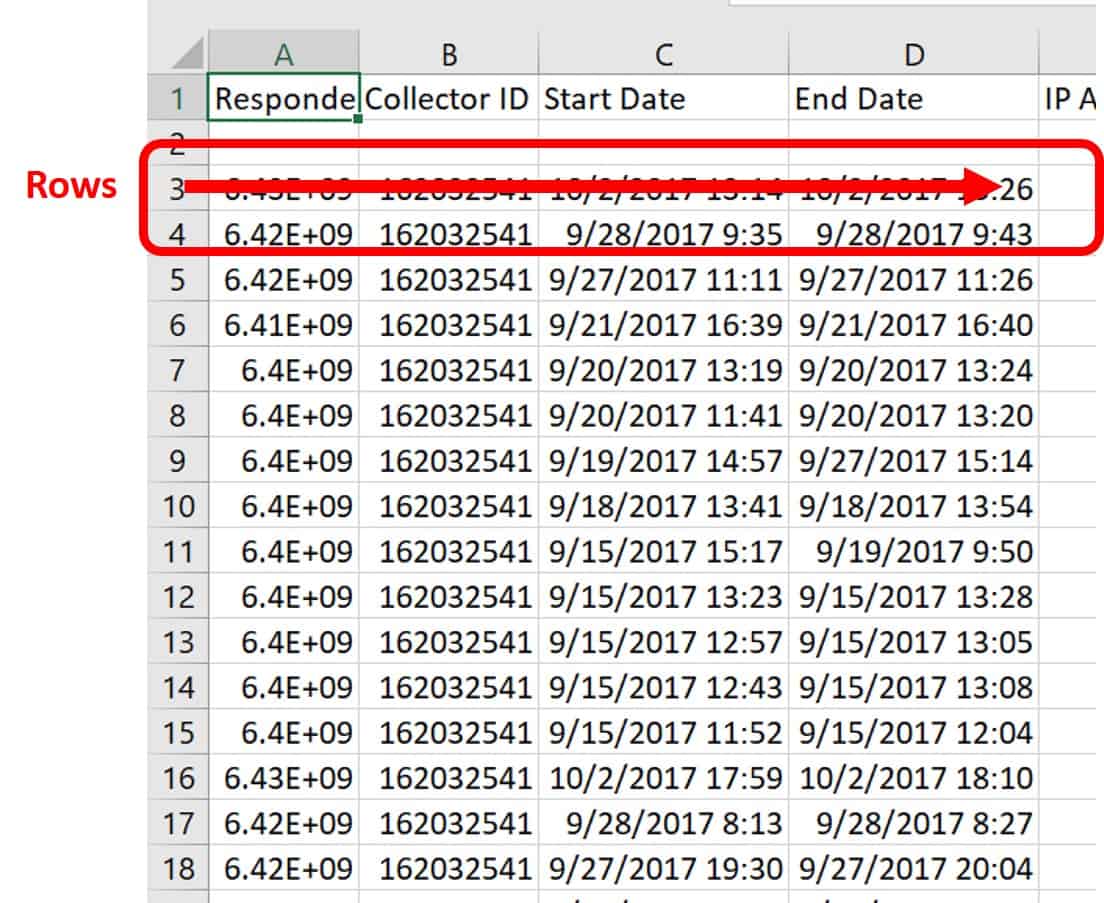
VLOOKUP is one of the logical functions in Excel, part of the lookup and reference functions for a database. A column in Excel is the vertical cells designated by a letter, while a row in Excel is the horizontal cells represented by a number, and a database is simply a list of data.

Follow these steps to use one of the preset formulas in Excel.

1. Click the Formulas tab.
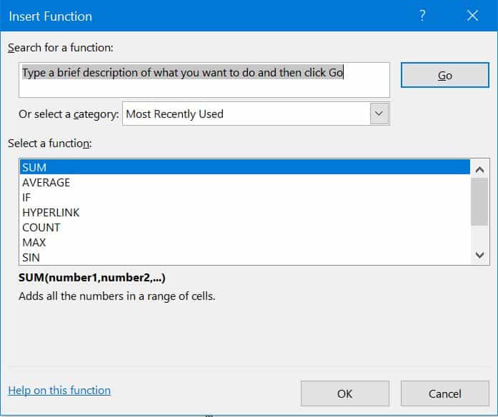
2. Click the Function (or Insert Function) icon on the far-left corner of the ribbon. Click on the formula you want to use (in our example, we’re choosing SUM), and click the OK button.
    
   
3. To add your own function, click on the designated cell and manually enter the formula.
   
   Some of the functions are basic, while others are more intricate. Examples of simple functions include those for basic arithmetic, such as the following:

*Both of these functions use operators, since there are not discrete functions for Excel.

More complicated functions can include nesting multiple formulas that give your sheet very specific utility. For example, you can nest SUMIFS and COUNTIFS formulas to evaluate your banking data and return the amount of money that your bank owes you. Once you master these functions, you can get very creative with Excel formulas when solving for the results you need.

Use VLOOKUP to find items within a table or a range of columns based on their row. The name VLOOKUP refers to looking something up vertically  – a value in your table – by matching on the first column. In other words, you are telling Excel a value you do know, and asking it to return a value that is related because it is in the same row but in a different column.

For example, you have a database of information about your staff. Each row lists a different staff member and lists data about them as it goes across. Column A is their name, column B is their employee ID number, column C is their desk phone number, and column D is the department. Finding Bob Smith’s phone number is not daunting when there are only 50 employees. You could easily do this visually. However, when you have 50,000 employees, it’s a bit more challenging. However, with VLOOKUP, you only need one piece of data, such as an ID number, to locate the rest of the employee information.

VLOOKUP often appears on resumes of people who interview for positions that require Excel skills. The VLOOKUP function comes standard in all modern Excel versions, from the 1997 version to the most current 2016 version.

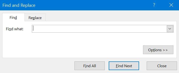
Normally when you search for a piece of data in a large spreadsheet, you press the Ctrl + F keys (a shortcut to open the Find and Replace box) on your keyboard. When the Find and Replace box appears on your screen, type in the item you are looking for in the Find what: field. Excel takes you to any exact matches in the spreadsheet.

You could then sort the spreadsheet to view the data you searched for. However, there may be many exact matches, so it could take a while.

The advantage of VLOOKUP is that it surfaces the data you are describing, not just the piece you know, and it performs this task without needing to sort the spreadsheet. You can also set VLOOKUP to run hundreds or thousands of matches at once, which saves you time rather than manually executing the task using the Ctrl + F function.

Additionally, you can add VLOOKUP in your more complicated formulas to present answers, not just pieces of data. For example, imagine you are ready to hand out bonuses to your sales team. There may be some new people that you are not yet ready to include, and you need a bottom line figure to present to your board for approval. The database tells you their current annual sales, annual salary, and how long they have been with the company. Using VLOOKUP with a few other relatively simple functions can surface the bottom line figure in a quick, easy formula.

Just as the name implies, the main use of the VLOOKUP function in Excel is to look things up, as listed vertically, whether you are looking for an exact match or an approximate match. You can also use the function on a data table with odd or non-intuitive codes in it. In Excel, you can add a new column that defines the codes and your VLOOKUP can fill in the data. Once you learn the basics, VLOOKUP is a simple function that is relatively easy to use. For example, the attached file lists salary information for 54 employees and can be used to follow along with the explanation below.

Let’s look at the composition of the VLOOKUP function. There are only four arguments in a VLOOKUP function – three are mandatory and one is optional. These arguments comprise the syntax of VLOOKUP.

In Excel, syntax means how you lay out your data, the order of your arguments, and how you write them. There are two ways to enter formulas in Excel. You can either enter them into a cell manually, or use the function wizard (shown above). Some experts disagree about whether the function wizard is the best avenue for inputting formulas. Whichever way you decide to input formulas is up to your comfort and experience level.

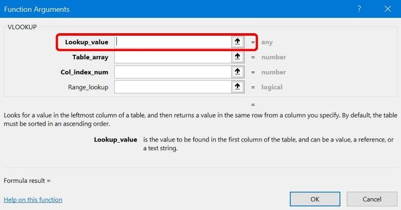
You can find the fields highlighted below by navigating to the function wizard and choosing VLOOKUP from the list of functions. Here are the the four arguments in VLOOKUP:

• Lookup Value: In the function wizard, this is the “What?” that you are trying to answer. This argument is mandatory.

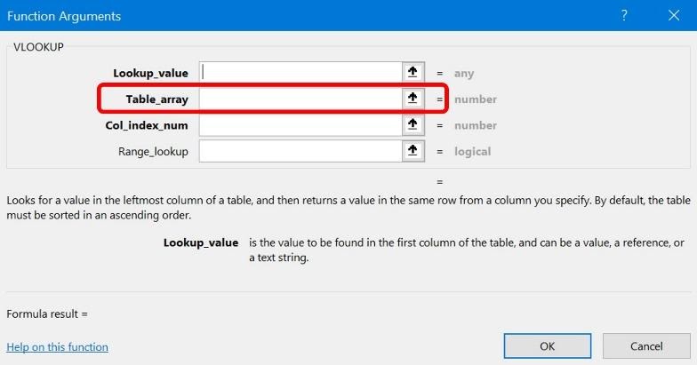
• Range: In the function wizard, the Table_array is where you will pull data from to answer your inquiry. This argument is mandatory.

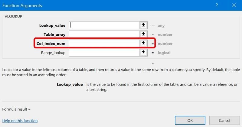
• Column Number: The Col_index_num in the function wizard tells Excel which column to pull the return data from. This is the third mandatory argument for VLOOKUP.

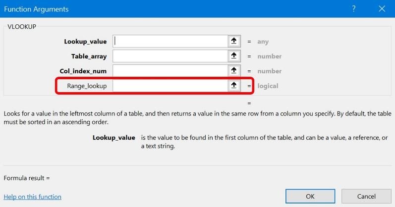
• True or False: This argument appears as Range_lookup in the function wizard. This is the last available argument, and is optional. Note: If you do not complete this box, the default is TRUE (or 1).

Putting the formula together,

VLOOKUP = (lookup_array, table_array, col_index_num, range_lookup)

Follow these steps to perform an Exact Match VLOOKUP in Excel.

1. Download the file Sample File for VLOOKUP Exercise.xls here.
    
   
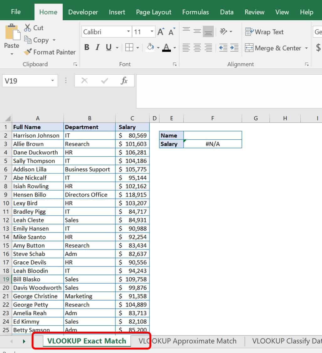
2. Click the VLOOKUP Exact Match worksheet tab.
   
   The tab includes a list of employees and their exact salaries. Although it’s not impossible to scroll and find the name and commensurate salary, a VLOOKUP formula is a quicker alternative. The function provides a quick, specific tool for each time you want to look up a salary, and is especially useful if you had thousands of employees in this list.
    
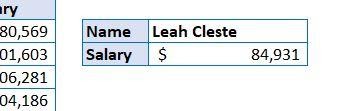
3. On the worksheet you’ll find a table that includes Name and Salary cells in column E. Type the full name of the employee, Leah Cleste, in the Name cell in column F, and the formula automatically fills in her corresponding salary below.

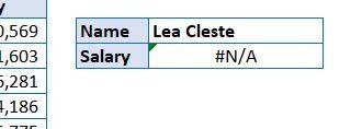
Since an exact match has been defined in the formula, you must fill in the name exactly as it is listed in the Full Name column (column A), without any misspellings. Otherwise, you will receive a #N/A error message shown below.

How to Perform an Approximate Match VLOOKUP in Excel

Follow these steps to perform an Approximate Match VLOOKUP in Excel.

1. Open the file Sample File for VLOOKUP Exercise.xls and click the VLOOKUP Approximate Match worksheet tab.

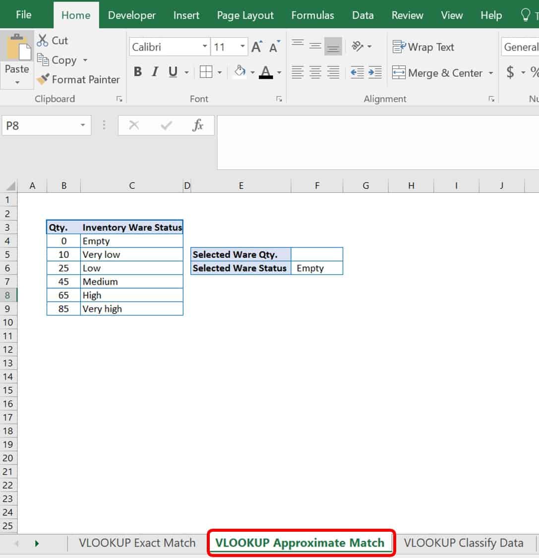
Try an approximate match instead of an exact match by inputting a value close to your lookup value such as one inside a numerical interval. This does not work well when your known value is text. In this example, you are looking for the ware status of your inventory. If you used an exact match VLOOKUP, you would only have a ware status when quantities were 0, 10, 25, 45, 65, and 85. However, because the formula dictates an approximate match, your categories are:
 

• 0-5 Empty
• 10-24 Very low
• 25-44 Low
• 45-64 Medium
• 65-84 High
• ≥85 Very high
   
  

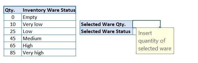
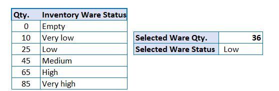
2. In this example, type the numerical value 36 in the Selected Ware Qty. cell in column F. The Selected Ware Status returned is Low. You should not receive any type of error message, regardless of the value you choose to insert. VLOOKUP provides the closest value to the category, without going into the next category.

An approximate match is the default functionality of VLOOKUP, and is used when you have a formula that does not specifically define either exact or approximate, which can happen when you don’t define the fourth argument in the formula.

Now that you’ve learned that VLOOKUP can find values in lists or tables, let’s look at other uses of VLOOKUP. Two alternative uses are data classification based on categories and joining data tables from separate sources based on a common data piece.

How to Classify Data Using VLOOKUP

Follow these steps to classify your own data using VLOOKUP

1. Open the file Sample File for VLOOKUP Exercise.xls.
2. Click the VLOOKUP Classify Data worksheet tab.

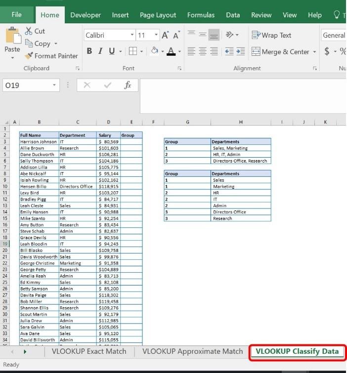
This is the same file of employees from above, but includes a Group column. In this example, you need to delineate your employees based on their group. Instead of using a complicated Nested If statement, you can use VLOOKUP to easily assign each employee a group.

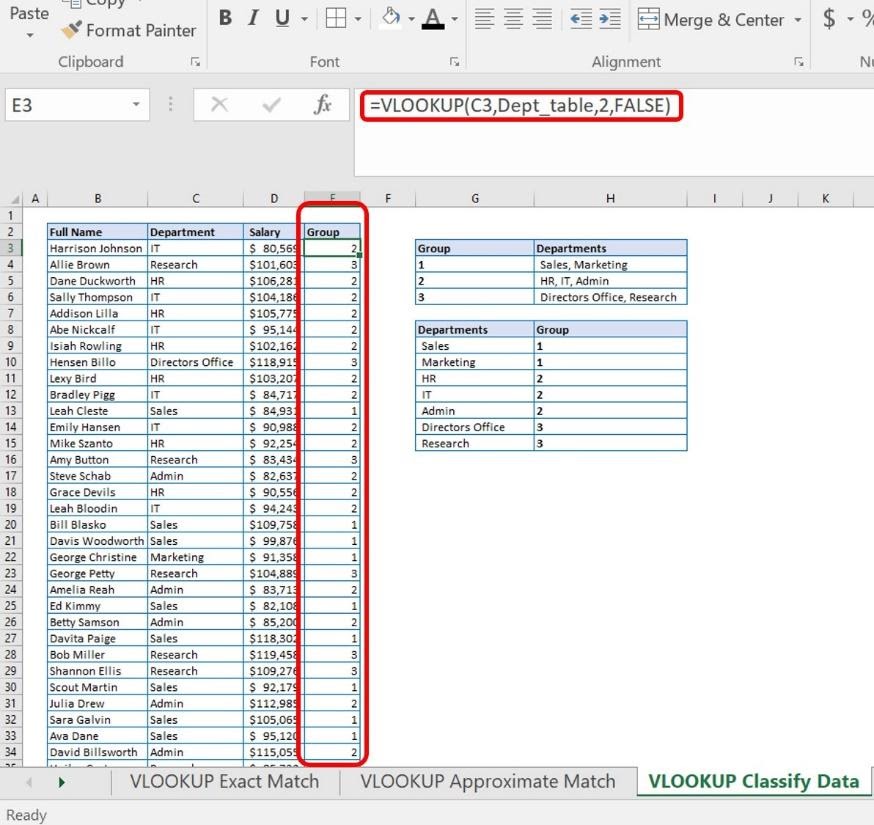
With a VLOOKUP formula added into column E (Group), you can assign each employee a group number based on the Department tables added in column H.

How to Join Data from Separate Sources

Follow these steps to join separate data tables into a single table using VLOOKUP.

1. Open the file Sample File for VLOOKUP Exercise.xls.

2. For this exercise, you’ll use two data worksheets. View VLOOKUP Join Data 1 and VLOOKUP Join Data 2.

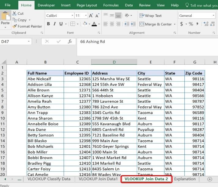
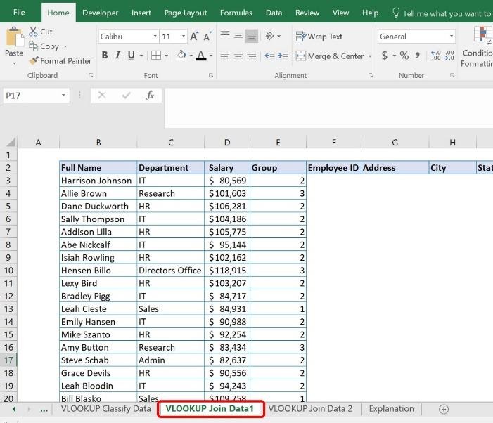
In this sample data, Full Name is in column B on both worksheets. This is the leftmost column of data in the data table. However, the VLOOKUP Join Data 1 sheet has different data for each employee than the VLOOKUP Join Data 2 sheet. The first worksheet has salary and department data, whereas the second worksheet lists their employee ID and personal address information. Since the two sheets have a common data piece (Full Name), you can use VLOOKUP to join them together quickly without performing complicated sorting and pasting. Full Name is the value that you are using to anchor your table.

3. Use the VLOOKUP Join Data 1 worksheet and add the columns from VLOOKUP Join Data 2 worksheet you want to see. In this case, add columns for Employee ID, Address, City, State, and Zip Code.

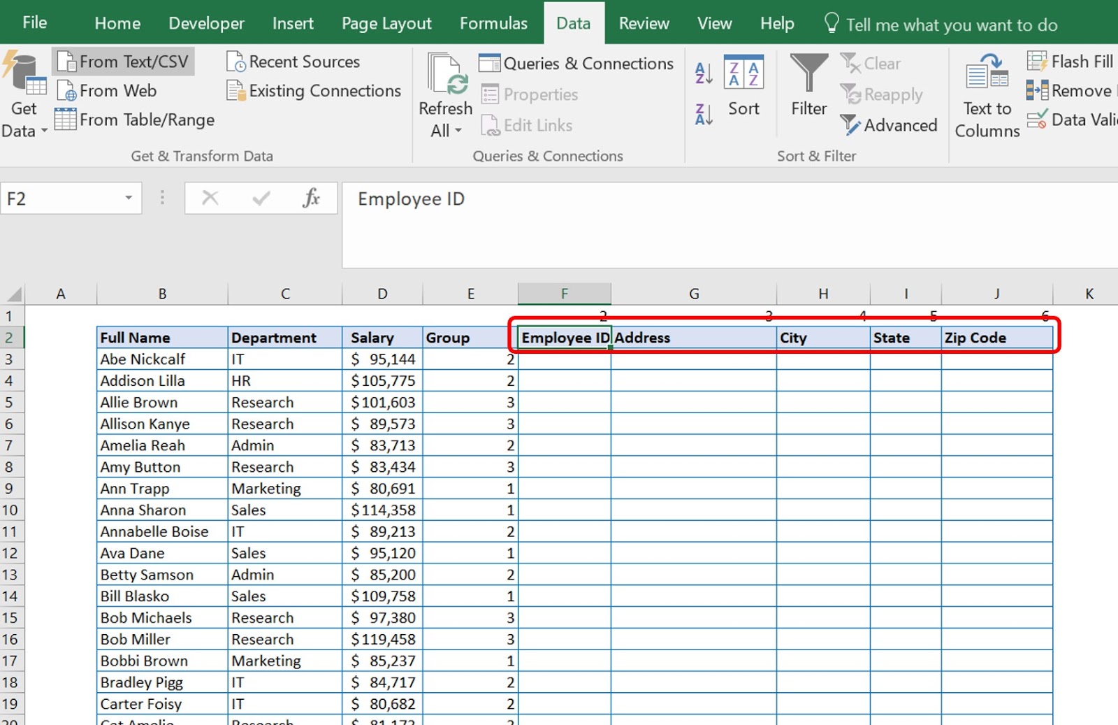
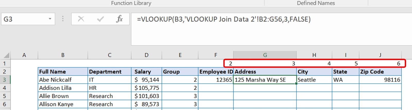
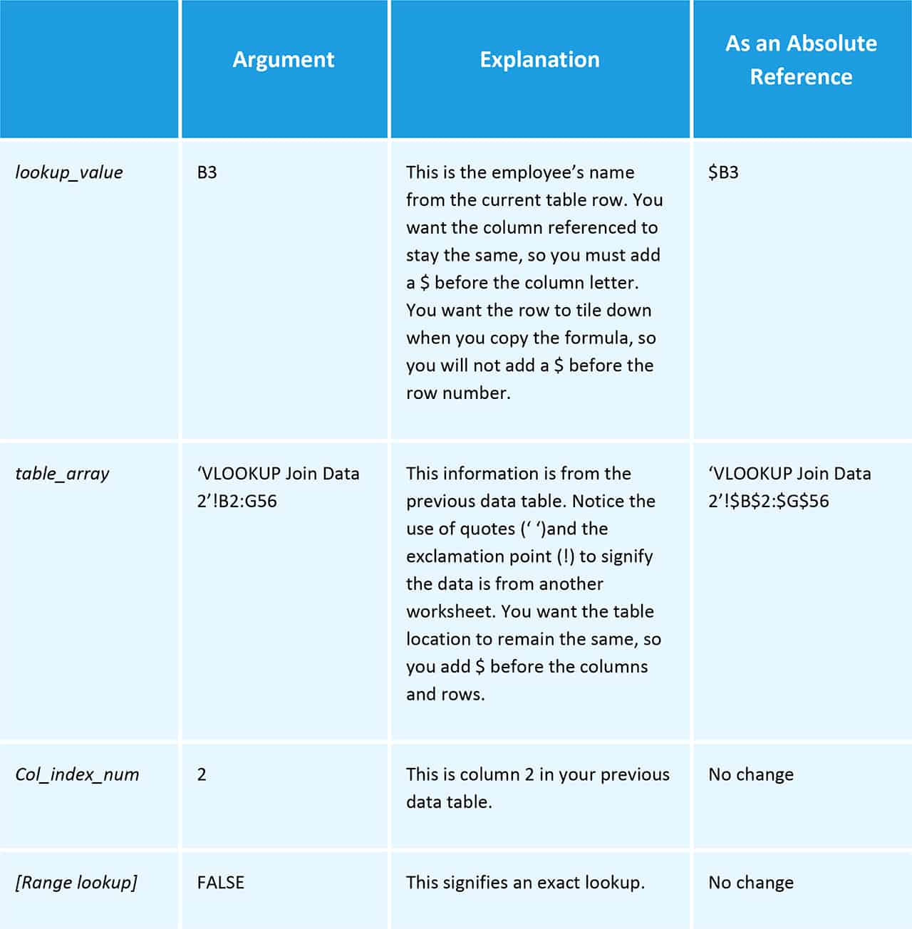
4. Add the first VLOOKUP formula in cell F3 for Employee ID. Add the following formula: =VLOOKUP(B3,'VLOOKUP Join Data 2'!B2:G56,2,FALSE).

The arguments are as follows:

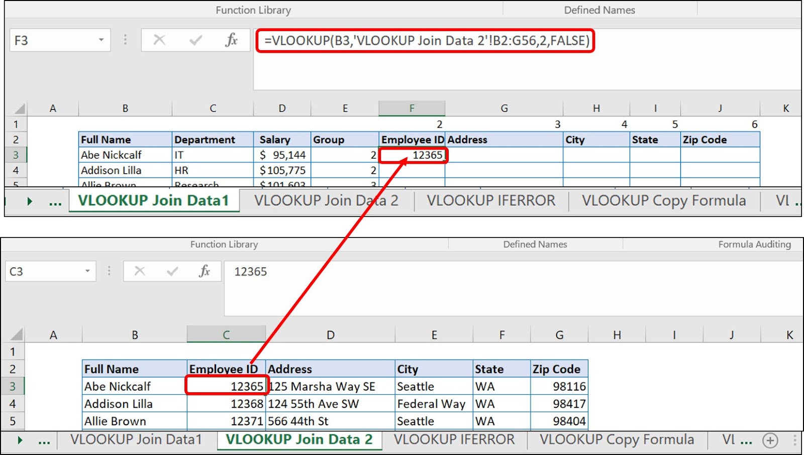
As you can see, the Employee ID from VLOOKUP Join Data 1 matches the Employee ID from VLOOKUP Join Data 2.

5. Add the VLOOKUP formulas for cells G3, H3, I3, and J3. These are the cells for Address, City, State, and Zip Code. The only change in the formula for their VLOOKUP is the column location number, as follows:

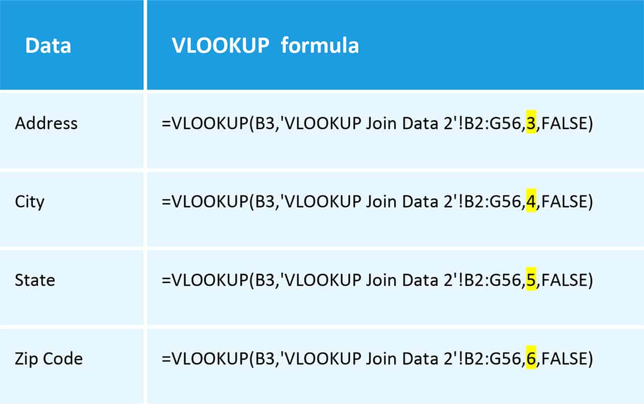
The numbers in the red box below represent the column location on the VLOOKUP Join Data 2 relative to the reference column, and match the change in the formula. They are merely a reminder for you as you type in your formulas.

6. Copy the five formulas you just typed across the row, cells F3, G3, H3, I3, and J3. Paste the formulas down through the rest of the table.

With a VLOOKUP formula added in to columns F through J, you have taken the data from VLOOKUP Join Data 2 and added it to VLOOKUP Join Data 1 to create one big table.

Before you start putting a formula together, look at the setup of your workbook. Some forethought can save you time and headache. Workbooks can get messy and lose utility when you place calculations haphazardly.

In the example below the authors have separated the data table and the VLOOKUP. There are defined borders that help you visually tell the difference between your data table and your VLOOKUP query. Decide how you want your query and your data tables to be visually delineated and set up your worksheet accordingly.

How to Enter the VLOOKUP Formula

Follow these steps to enter your own VLOOKUP formula using the syntax above.

1. Click the cell where you will type your formula. For this example, you will use the same VLOOKUP Exact Match worksheet used earlier to match the salary for your named employee. Therefore, you will put the VLOOKUP formula in the cell where you want to see your retrieved information. Click on that cell.

2. Type =VLOOKUP (to signal to Excel that you are creating a VLOOKUP formula. Excel will open a tool tip box to help you keep track of the arguments while writing the formula. The bolded portion is the required argument you need to enter. Between each argument, type a comma (,) with no spaces.


 

3. Type in the lookup_value. For this example, the lookup value is cell F2, which represents the value in the database that you know – the Full Name of the employee.

The dollar signs ($) before the F and before the 2 stand for an absolute or anchored value. Normally, when you copy and paste cells with formulas in them, Excel shifts the formula relative to the new position.

For example, if you have a simple formula such as =A1 located in cell B1 (as in the diagram below) without the dollar signs, and you copy/paste the cells down the column, the value in B2 becomes A2, B3 is A3, and so on. When you include the dollar signs in the formula (as shown in the second diagram) the value of all the pasted cells pasted is the same as what’s in cell B1. In other words, when you put a dollar sign before the column letter, you are telling the formula to stay with the original column location. When you put the dollar sign before the row number, you are telling the formula to stay with the original row number. This can be helpful as you use more complicated formulas and forms.

4. Next, type in the range – the table_array. This tells Excel where you are looking for data. For this example, this is the data table from A1:C55. You can either type the parameters of the table into the formula or select and highlight the whole table to have Excel load it into the equation.

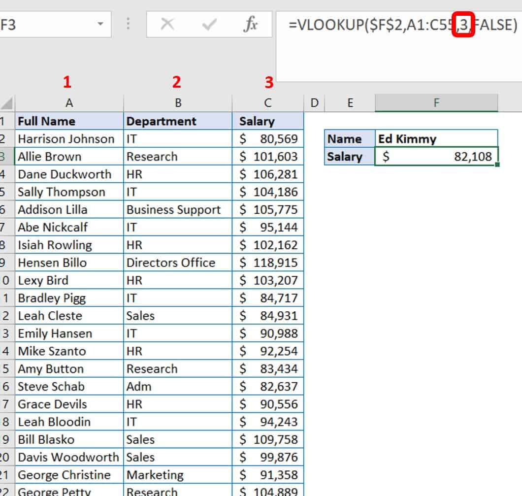
5. The next argument concerns which vertical column you want Excel to look in that correlates with the value in the location you identified. This is your col_index_num, and in this example, should be 3 to represent how many columns from column 1 (the leftmost column on the sheet). In other words, you are telling Excel to first look at the value in F2, and then find that value within the table located from A1:C55. Excel should move three columns over and return the value located in that cell. So far, the VLOOKUP formula looks like this:

6. Decide whether the data needs to be exact or approximate. As discussed above, the vast majority of scenarios will require exact answers. It would be inappropriate to look for George Christine’s salary and have George Petty’s salary populate. This is the fourth argument [range lookup] in this formula. The default is TRUE for this, which is an approximate match. You may also enter 1 for an approximate match. FALSE is an exact match. You may also enter 0. As you can see in the image below, Excel tries to help you type the right formula and provides a pop-up box as you start typing that reminds you of the difference between these values.

Now, you can check your formula. Input correctly, you should see the correct salary when the employee name cell is updated. For example, Harrison Johnson should have a salary that populates as $80,569. If Harrison’s salary comes up as $95,144, then you have not chosen the correct range lookup value.

You will find a step-by-step guide to performing a VLOOKUP for Excel 2010 here.

You will find a step-by-step guide to performing a VLOOKUP for Excel 2013 here.

You will find a step-by-step guide to performing a VLOOKUP for Excel 2016 here.

VLOOKUP is one of the most common functions to return #N/A errors in Excel when set up improperly. VLOOKUP returns an #N/A error when it cannot find a referenced value.

Since approximate matches are considerably less prone to return #N/A errors, the first assumption is that you are using VLOOKUP to return an exact match. There are several reasons your VLOOKUP can return an #N/A error, including:

If you are using a formula with an approximate match:

Many people do not like displaying #N/A errors, especially when designing template forms. If you receive an #N/A error in an exact match VLOOKUP, you can have your VLOOKUP display a another message or a blank cell. This is called “trapping” an error. The easiest way to trap this error and display something friendlier than a #N/A error, such as “Not found” or even “0”, is to wrap your formula with an IFERROR formula.

How to Enter an IFERROR Formula

Follow these steps to wrap your VLOOKUP with an IFERROR formula.

1. Open the file Sample File for VLOOKUP Exercise.xls and click the VLOOKUP IFERROR worksheet tab.
   
    
   
   
    
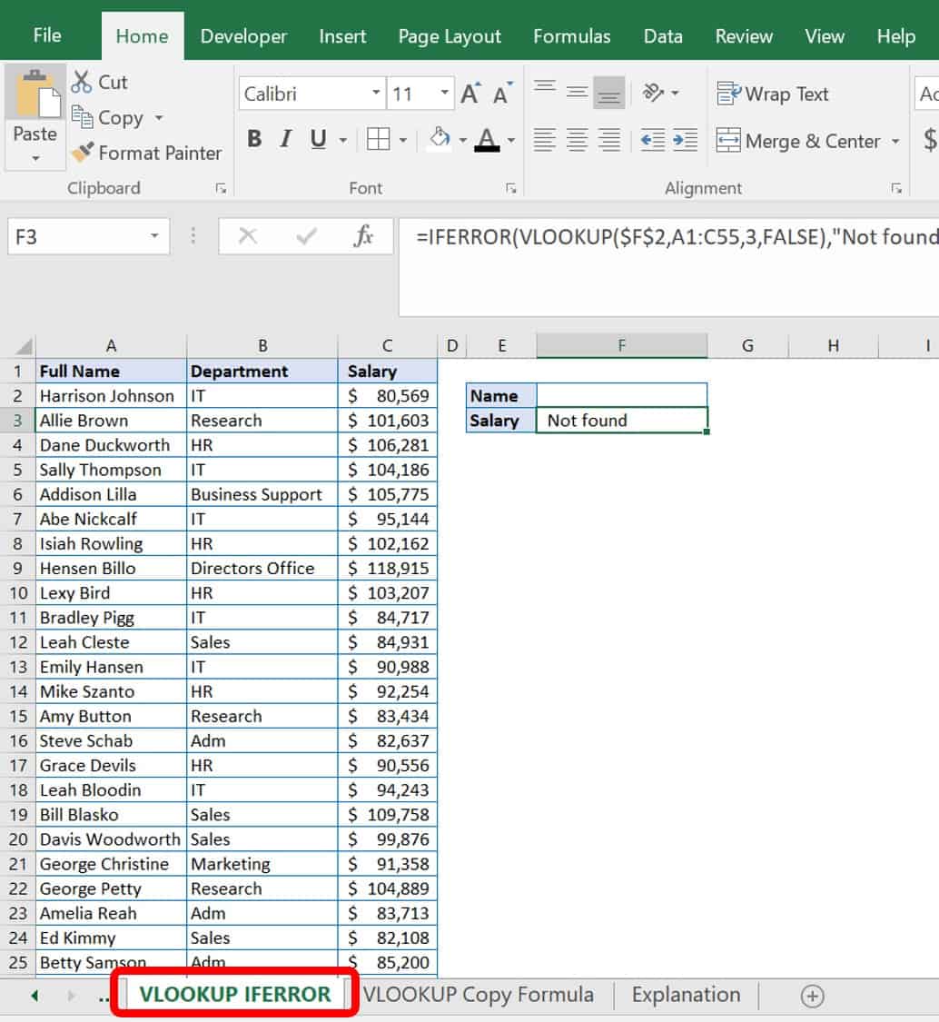
2. Add parentheses around the original VLOOKUP formula, and type IFERROR after the equal sign (=). After the VLOOKUP formula, add a comma (,), and then in quotes (“ “) add your friendly message. If you would like nothing to show in the cell, enter quotes (“”) only. In the example here, we added “Not found” to appear when an employee name is not in the table.

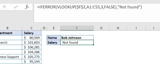
The original VLOOKUP formula was =VLOOKUP($F$2,A1:C55,3,FALSE). With IFERROR wrapped around it, the formula is now =IFERROR(VLOOKUP($F$2,A1:C55,3,FALSE),”Not Found”).

Instead of typing in a new VLOOKUP formula for every row in a table, you can simply copy the original VLOOKUP formula. In this case, you must use absolute cell references ($), as discussed earlier, for the data pieces that you do not wish to change in the formula.

Follow these steps to copy your VLOOKUP formula.

1. Open the file Sample File for VLOOKUP Exercise.xls and click the VLOOKUP Copy Formula worksheet tab.
   
    
   
   
    
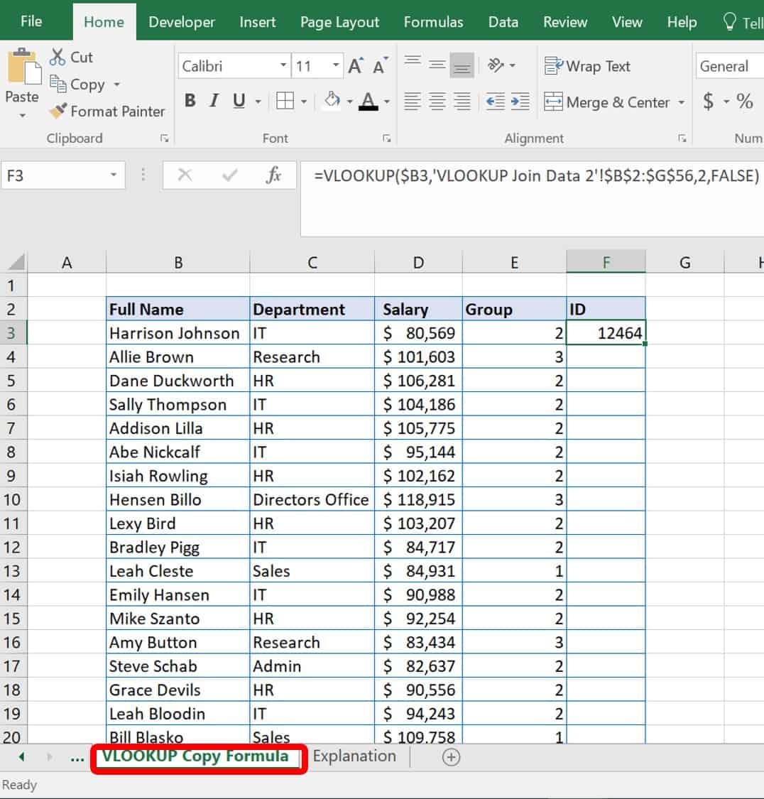
2. In this example, copy the VLOOKUP formula located in cell F3 into the rest of the column to populate all the correct IDs. However, first check that the VLOOKUP formula has absolute values in place. In this case, you want to make sure that you can copy your formula and paste it down the ID column.
3. The VLOOKUP formula used to populate your staff’s ID numbers comes from the data in the VLOOOKUP Copy Formula worksheet and from the VLOOKUP Join Data 2 worksheet.
   
   
    
   
   
    
4. Review the VLOOKUP formula for the first staff member in the table, Harrison Johnson. The formula should be:
   
   =VLOOKUP(B3,’VLOOKUP Join Data 2’!B2:G56,2,FALSE)
   
   where the arguments are as follows:
   
    
   
   
    
5. A shortcut to add absolute references to your formula values is to select the formula portion and click F4, which adds the $ to your formula. The first click will add the $ to both the column and row. Click F4 again to add $ to just the row number, and click a third click time add $ only to the column letter.
6. Copy your VLOOKUP formula in cell F3.
7. Select the remainder of Column F within your table.
8. Click Paste.
9. Click Enter. See the result in the image below.
    

This is one of the more confusing, but surprisingly simple, arguments in a VLOOKUP function. The Column Index Number represents how many columns from the left-most column that you want Excel to search within and return a value. Regardless of how complicated the remainder of your formula gets, your col_index_num is always a simple integer, greater than or equal to 1.

In this example, there are three columns (Full Name, Department, and Salary). You are looking for an employee’s salary, so enter 3 for the col_index_num. If you  entered 1, the formula would return the employee’s full name. If you entered 2, the formula would return the employee’s department.

Often, when importing data into Excel from other databases, you run into the problem of leading or trailing spaces. This is especially true of accounting systems. For the leading spaces, consider either using Text to Columns or the TRIM function. For trailing spaces, you can use either the TRIM function or add wildcards into your VLOOKUP function. The simplest fix is adding wildcards.

Wildcards are characters that tell Excel that you are not exactly sure what you want to fine. You may use certain strings or characters to search for something. There are two key types of wildcards in Excel: the question mark (?) and the asterisk (*). Use the question mark in exchange for any single character. For example, “B?ll” returns “Bill” or “Bull”. Use the asterisk in to exchange one or more number of characters. For example, “South*” returns “South”, “Southwest”, or “Southeast”. Using “(*)” returns anything enclosed by parentheses.

You may want to search for a staff member named “Betty” in your Excel database, but match against all possible outcomes, including “Betty Peterson”, “Betty Norris”, and “Betty Samson”. To do this search, you can use the wildcard character.

How to Use Wildcards in a VLOOKUP

Follow these steps to use a wildcard in your VLOOKUP formula.

1. Open the file Sample File for VLOOKUP Exercise.xls.

2. Click the VLOOKUP with wildcard worksheet tab. You will also use the Export_PayToDate worksheet. In this scenario, you have exported data from your accounting system (Export_PayToDate).

Perform a VLOOKUP of this accounting data to update column E (Paid To Date) in your VLOOKUP with wildcard worksheet. Since this data is coming from your accounting system, there are numerous trailing spaces. For example, the column A exported label is “Full Name.                 “ (see how it includes a bunch of trailing spaces).

Since the lookup value does not have the trailing spaces, you will get an “#N/A” error. Using exact match logic, and a lookup value with no trailing spaces, means your query does not match any of the lookup column values because they contain trailing spaces from your accounting system’s export.

3. Wildcard characters work within the VLOOKUP function when you meet two conditions. The lookup value must be a text string, and the fourth argument must indicate exact match logic. Since both of these conditions are met in the example, you would choose a wildcard based on the extraneous spaces, which is the asterisk.

4. Using the concatenation operator (&), join the lookup value in the VLOOKUP formula with the asterisk (*).

The original formula was:

=VLOOKUP(B3,'VLOOKUP with wildcard'!A1:G55,6,FALSE)

With the wildcard concatenated in, add &”*”  into the lookup value:

=VLOOKUP(B3&”*”,'VLOOKUP with wildcard'!A1:G55,6,FALSE). B3&”*”
 

That’s the lookup value, the value in B3 and the * wildcard. When added to the spreadsheet, you’ll see this result:

Experts consider one of VLOOKUP’s shortcomings to be that it only matches on the first instance of your lookup value, and does not make allowances for duplicate values. You could choose to remove the duplicate values and use a unique lookup value; however, there is another way to handle duplicate values that is less manual.

How to Handle Duplicate Values in Excel Using VLOOKUP

Follow these steps to find duplicate values with VLOOKUP.

1. Open the file Sample File for VLOOKUP Exercise.xls.

2. Click the VLOOKUP Duplicate Values worksheet tab. Notice that this is a subset of your staff salary table. However, you have two employees with the same name, John Smith. Fortunately, they work in different departments and since you know about this issue, there is a workaround you can use to separate your John Smiths and retrieve the correct information.

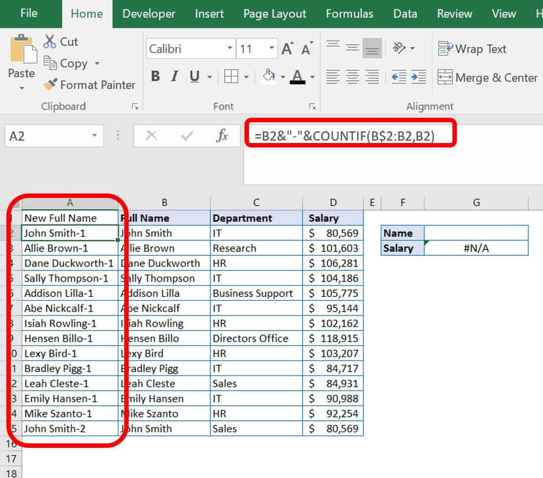
3. Right-click column A and click Insert for a new column. This column will be added to the left of the Full Name column.

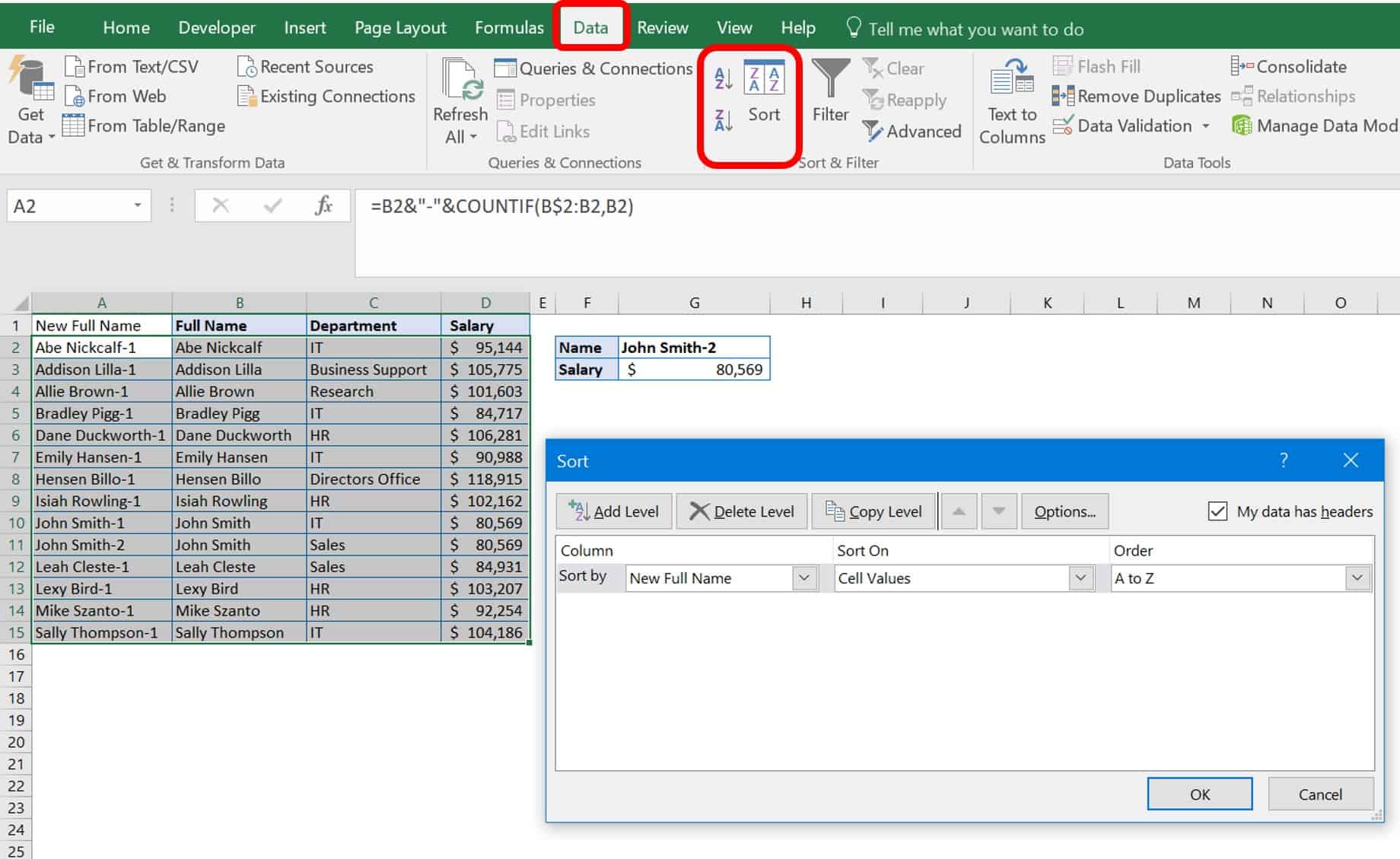
4. Add a reference, a concatenate, and a COUNTIF formula together in a new cell A2.

This looks like =B2&”-“&COUNTIF(B$2:B2,B2).

Each formula part means:

5. Sort your data table to view duplicates side by side. Select your data table. Click the Data tab. In the Sort & Filter menu, click Sort. Click the checkbox “My data has headers” and ensure the following are showing:

Column     New Full Name

Sort On    Cell Values    

Order         A to Z

Click the Ok button. Now your John Smiths are next to each other, but delineated by a dash and a number 1 or 2.

​

6. Check your VLOOKUP formula to ensure that it matches the current data table parameters. Since you added a column, you will need to update the VLOOKUP to reflect its presence. The formula should now read:

=VLOOKUP($G$2,A1:D15,4,FALSE).

In software programming, a self-contained system (SCS) is one whose functionality exists in independent systems. Although not a ubiquitous term, self-contained in the field of program functionality means that your formula is not looking at other code elsewhere. In Excel, a self-contained VLOOKUP means that your formula is looking inside itself, not in a separate table to find the lookup value.

You can perform a self-contained VLOOKUP as either an exact or approximate match. You have already learned that your VLOOKUP formula has four parts: lookup value, table_array, col_index_num, and [range lookup]. So to make a formula self-contained, somewhere in these arguments must exist all the values you will need for lookup. The simplest way is to turn your table array into an array constant. An array constant is the set of values you need within curly brackets {}.

How to Write a Self-Contained VLOOKUP Formula

Follow these steps for a self-contained VLOOKUP.

1. Open the file Sample File for VLOOKUP Exercise.xls and click the VLOOKUP Self-Contained worksheet tab.
2. Set up your chart. In this example, there is a two-column chart with room to enter a score and the letter grade filled in by the VLOOKUP formula.
3. Enter the VLOOKUP formula with your four arguments. For the table_array however, enter an array constant. What would normally be a range of cells such as C5:D25 should look like {integer, “label”; integer, “label”…}. This array separates the elements by a comma between each related value and a semicolon before the next related pair. The whole array is captured between curly brackets {}. You do not need to click Ctrl+Shift+Enter as you would in an array formula. For this example, the formula reads:

=VLOOKUP(B3,{0,"E";62,"D";75,"C";83,"B";92,"A"},2,TRUE)

So far, we have covered the glaring VLOOKUP errors and how to fix them. However, you can adhere to data table set-up best practices to avoid errors in the first place. These include:

Generally, Excel displays the #VALUE! Error if the formula uses the wrong data type. A #VALUE! is Excel’s way of telling you that there is something wrong with the formula you have typed or the cells you referenced. The chart below offers the three most common reasons you will get a #VALUE! Error and how to fix them:

Now that you know how to set up a VLOOKUP formula, the following list has pointers to help you remember how to set it up in the future. So, remember this:

• VLOOKUP retrieves data based on a column number.
• VLOOKUP always finds the first match.
• VLOOKUP is case-insensitive.
• VLOOKUP has two matching modes: exact and approximate.
• VLOOKUP uses approximate match by default.
• Named ranges make VLOOKUP formulas easier to read when writing them.
• Use a separate worksheet for your database tables.
• You can use ROW or COLUMN to calculate a column index.
• You can use VLOOKUP to replace nested IF statements.
• VLOOKUP can only handle searching for a single criterion.
• Use F4 within the formula (cursor needs to be on a cell range) to make your cell references absolute.
• Two VLOOKUPS are faster than one VLOOKUP

There are other functions in Excel that are similar to VLOOKUP and also functions that perform almost the same job as VLOOKUP. For example, HLOOKUP is similar because it looks up and retrieves data, but it does so based on horizontal placement in a table or list. Instead of looking down in the table, the formula specifies moving horizontally to the right. Your choice of function is based on how the original table is set up.

As you can see, the data in this table is a portion of our employee data, but arranged horizontally across the page. You can perform the same lookup function, only with a small tweak of using the HLOOKUP function.

INDEX and MATCH are two other functions that when performed together have the same functionality as VLOOKUP. These functions tell Excel what array (or data set) to look at, and where to match data from and to.

As you can see from the example, we found the salary of Allie Brown using the same data setup as our VLOOKUP, but with a combination of two different functions. Some experts say that INDEX- MATCH has better functionality than VLOOKUP for the following reasons:

• Insert or Delete Columns Without Breaking Your Formula: In VLOOKUP, if you delete or insert extra columns, your formulas will need to be updated because you change where your formula looks for data. The column number you specify in your VLOOKUP formula changes if you add or remove a column.
• VLOOKUP Only Looks Right: In VLOOKUP, Excel cannot look right and left. The lookup value must always be in the left-most column. This requirement does not limit INDEX-MATCH.
• VLOOKUP Processes Slower: With small tables, you would hardly notice slow processing. However, with hundreds or even thousands of rows of data, VLOOKUP is slower than INDEX-MATCH because it must search every row of data. INDEX-MATCH looks only at the specified row and column.
• VLOOKUP Has a Character Limit: VLOOKUP only allows you to have 255 characters in your lookup criteria, or it will return an error. INDEX-MATCH can lookup character strings that are longer than 255 characters.

Empower your people to go above and beyond with a flexible platform designed to match the needs of your team — and adapt as those needs change. 

The Smartsheet platform makes it easy to plan, capture, manage, and report on work from anywhere, helping your team be more effective and get more done. Report on key metrics and get real-time visibility into work as it happens with roll-up reports, dashboards, and automated workflows built to keep your team connected and informed. 

When teams have clarity into the work getting done, there’s no telling how much more they can accomplish in the same amount of time. Try Smartsheet for free, today.