What Is the Formula for VLOOKUP in Excel?
In Excel, VLOOKUP is a lookup/reference function that helps you find an item in a table or range of cells vertically by their row. Four arguments comprise the syntax of the VLOOKUP function; the arguments are the value you want to use as a reference, the range or table of cells that hold the value you seek, the column number for your return value, and whether you want an exact or approximate match. Respectively, these arguments in the VLOOKUP formula are lookup_value, table_array, col_index_num, and [range_lookup].
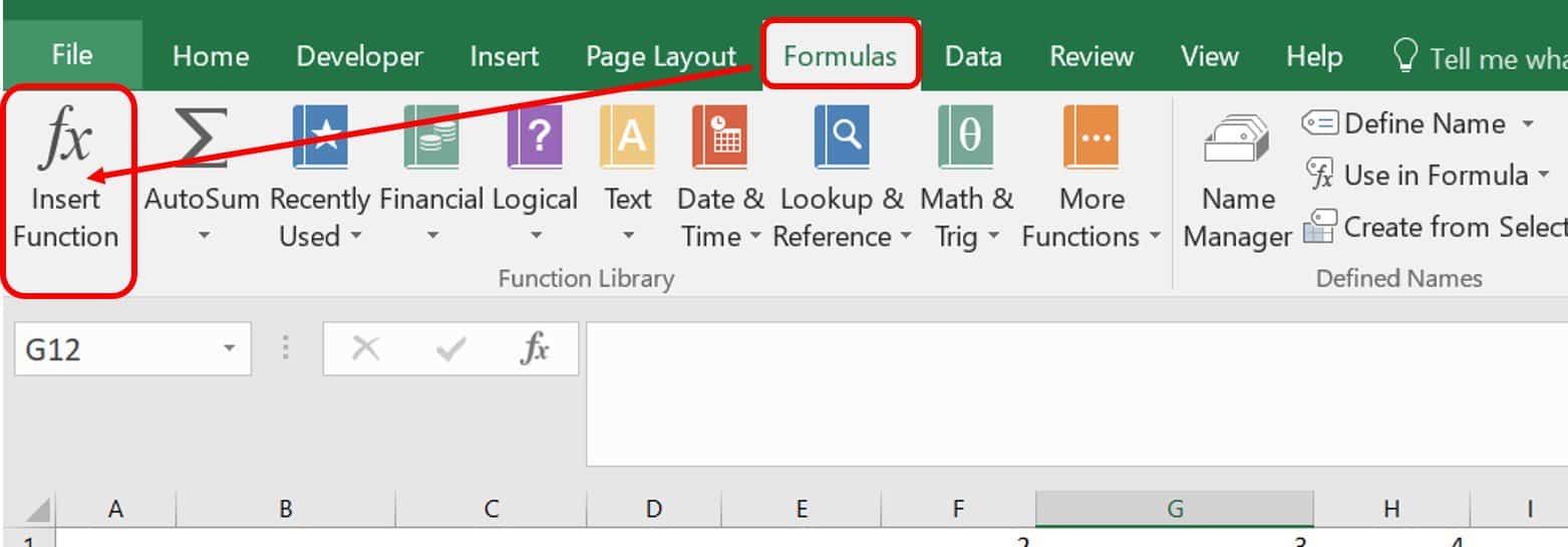
There are two ways to input formulas in Excel: You can type the formula directly in the cell or use Excel’s Formula Wizard.
Follow these steps to use Excel’s Formula Wizard for a VLOOKUP function.
- Click the Formulas tab.
- Click the Insert Function icon on the top-left corner of the ribbon.
- When the Insert Function box appears, type vlookup into the search box, and click Go. Click OK.
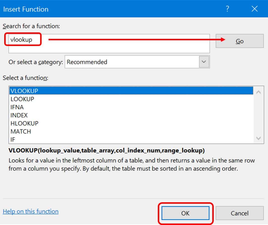
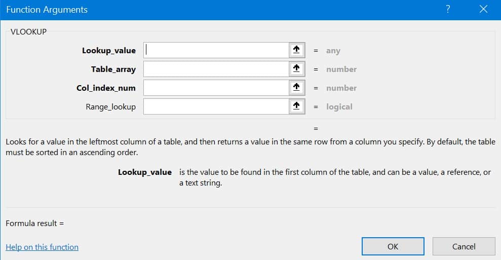
The Functions Argument box will then appear, which walks you through inputting the VLOOKUP formula.
How VLOOKUP Works
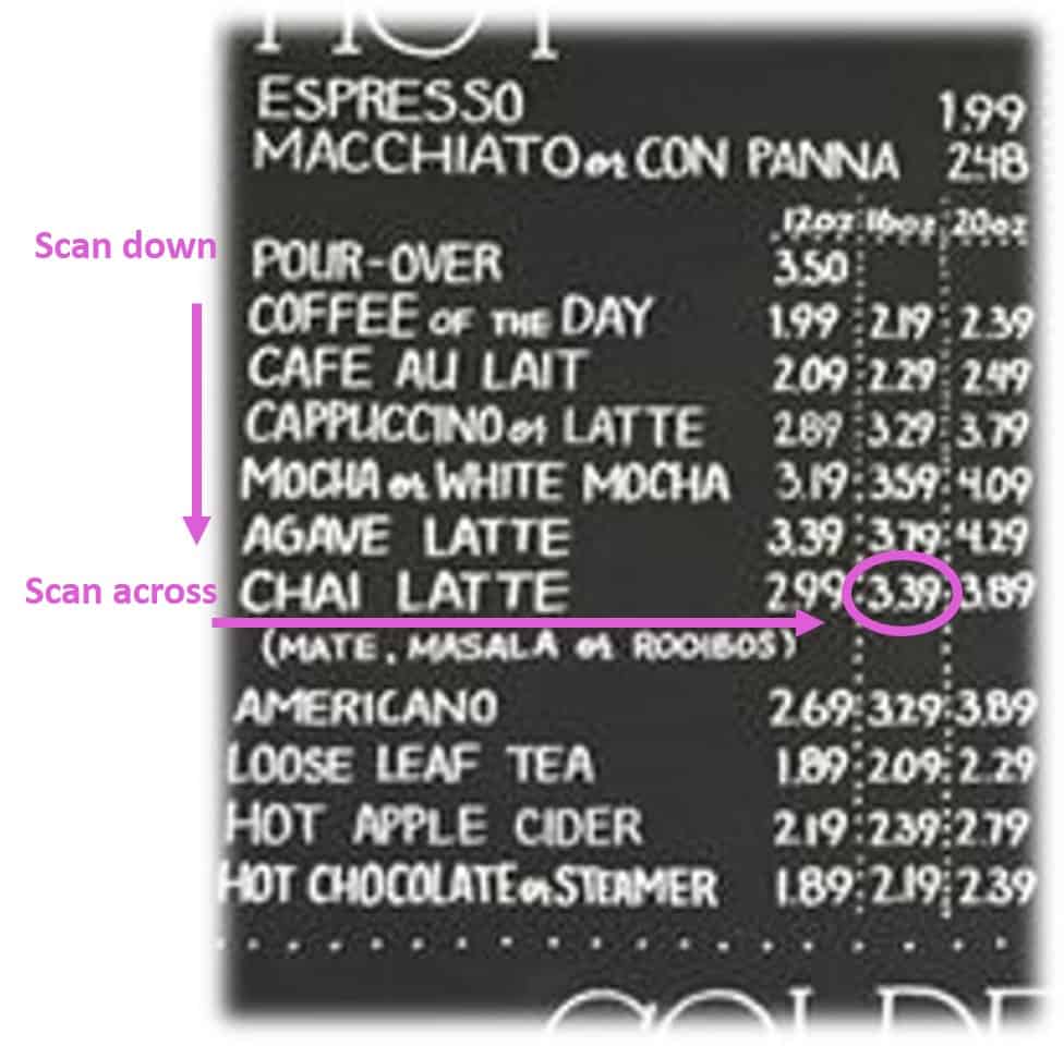
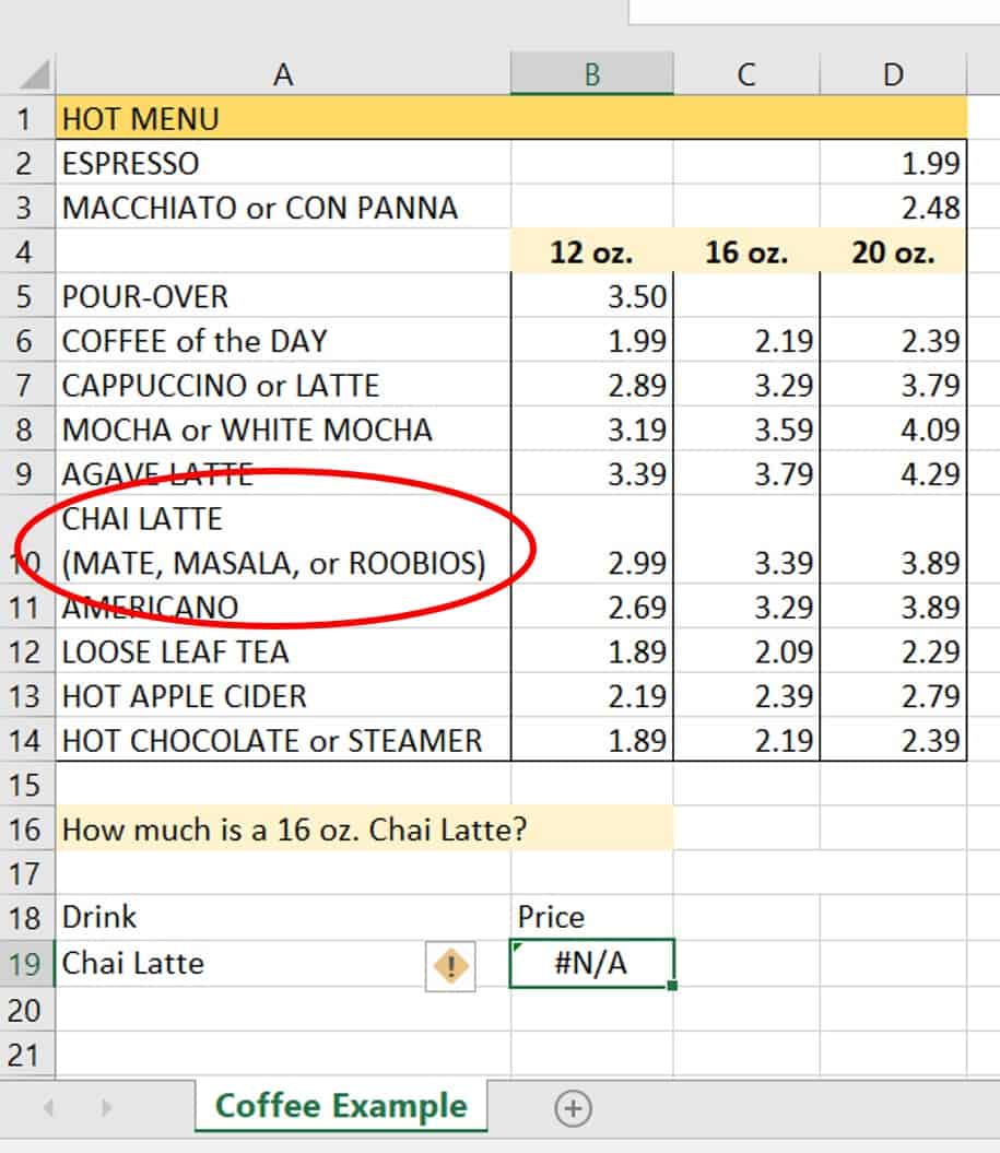
To understand how VLOOKUP works, let’s use your favorite coffee order. The menu for your coffee shop is a good example of how you often perform a version of VLOOKUP in your head, scanning across from your drink of choice to the price under the preferred size of your drink.

In Excel, VLOOKUP scans the cell in the data table and looks for the data and the location you specify. When you hone in on the Hot menu, you see that there are three columns (sizes): 12 oz., 16 oz., and 20 oz. If you were ordering a 16-oz. chai latte, you would scan down the column of drinks until you find the chai latte, then across the row until you stop at the price in the appropriate (16 oz.) column. From there, you would determine that the drink costs $3.39. This process is not much different from what happens in Excel using the VLOOKUP function.
VLOOKUP Example: How to Perform an Exact Match
We’ll use the same coffee example in Excel. Download the Excel Sample Data file to follow along. A note about the sample file: All the data you need for the majority of the examples explained throughout this tutorial are included in the file. Simply scroll through the tabs to find the corresponding example. Some worksheets already have the VLOOKUP formulas completed in the cells noted in the tutorial. To do it yourself, delete the existing formula and enter the one in this tutorial.
In the Excel worksheet, you can scan down the column to find chai latte, then across to the column for 16 oz. However, because the majority of Excel spreadsheets will not be a simple coffee order, Excel provides functions to help you look up your data. In this example, you could use VLOOKUP to determine the cost of your 16-oz. chai latte. Follow these steps to perform an exact match VLOOKUP in Excel.
- Click the Coffee Example worksheet tab in your sample workbook.
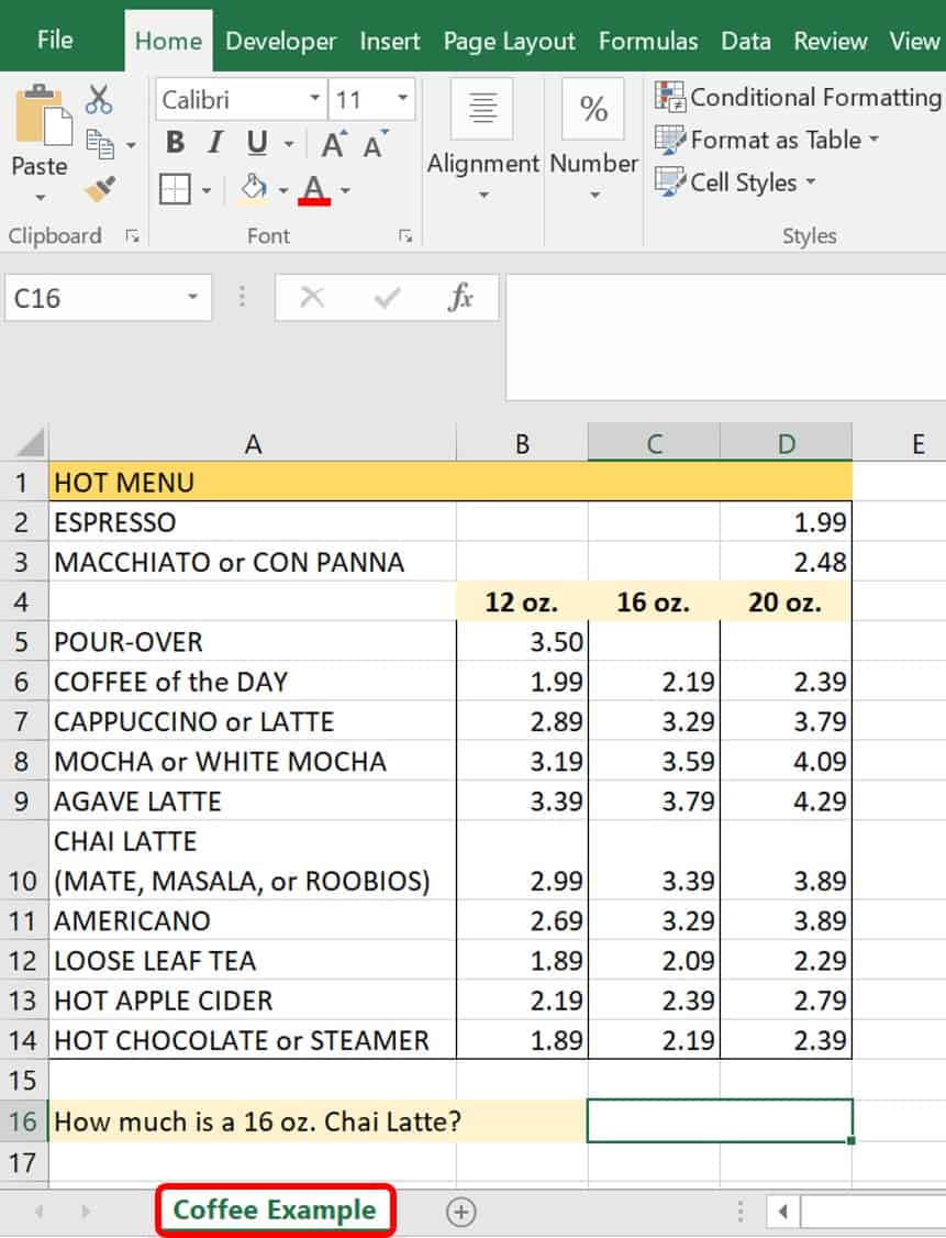
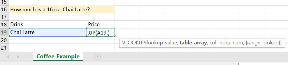
- On the worksheet, you see the same Hot menu from the coffee shop blackboard image above. Use the VLOOKUP function, and click cell B19, where you will enter your formula.
- Type =VLOOKUP (to let Excel know that you are creating a VLOOKUP formula) in the formula bar. Excel will open the tool tip box to help you keep track of the components of the formula. As you enter your formula, Excel bolds the portion you are inputting in the tool tip box to help you track the calculation.

- Type the first argument, lookup_value, as cell A19, which has the value you want to look up. By placing this value outside of your data table (menu), you can change the data and still have the correct results when you look up a value. Type a comma (,) between each argument.
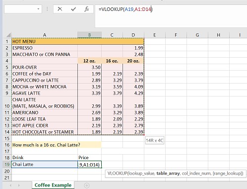
- Type the second argument, table_array. This is the entirety of your data table. You can manually type A1:D14, or you can use your mouse to highlight the cells on the table and Excel populates its parameters into the formula. Type a comma (,).
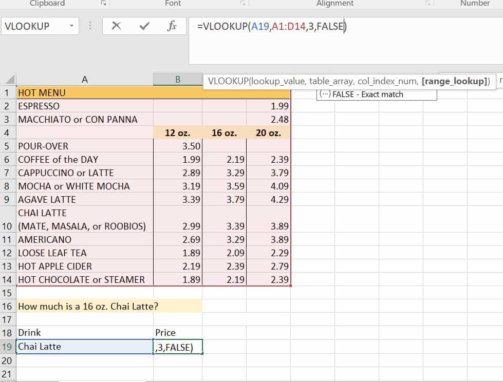
- The next argument is col_index_col. This is the column number in the data table that you are scanning to get to the row hosting the piece of data you defined in the first argument. In other words, in the first argument, you told Excel what data piece it was looking for: in this case, “Chai latte”. This defines where Excel should start. In the second argument, you told Excel the parameters of the data table. Now that you’ve defined the data table parameters, you are telling Excel which column to scan for your answer. In this case, enter 3. This is the third column from the lookup values. The lookup values must always go in the first column. Then type a comma (,).
- The last VLOOKUP argument for an exact lookup is [range_lookup]. Type FALSE or 0. Your lookup will now be exact.
- Type a close parenthesis ) and click Enter on the keyboard.
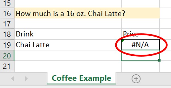
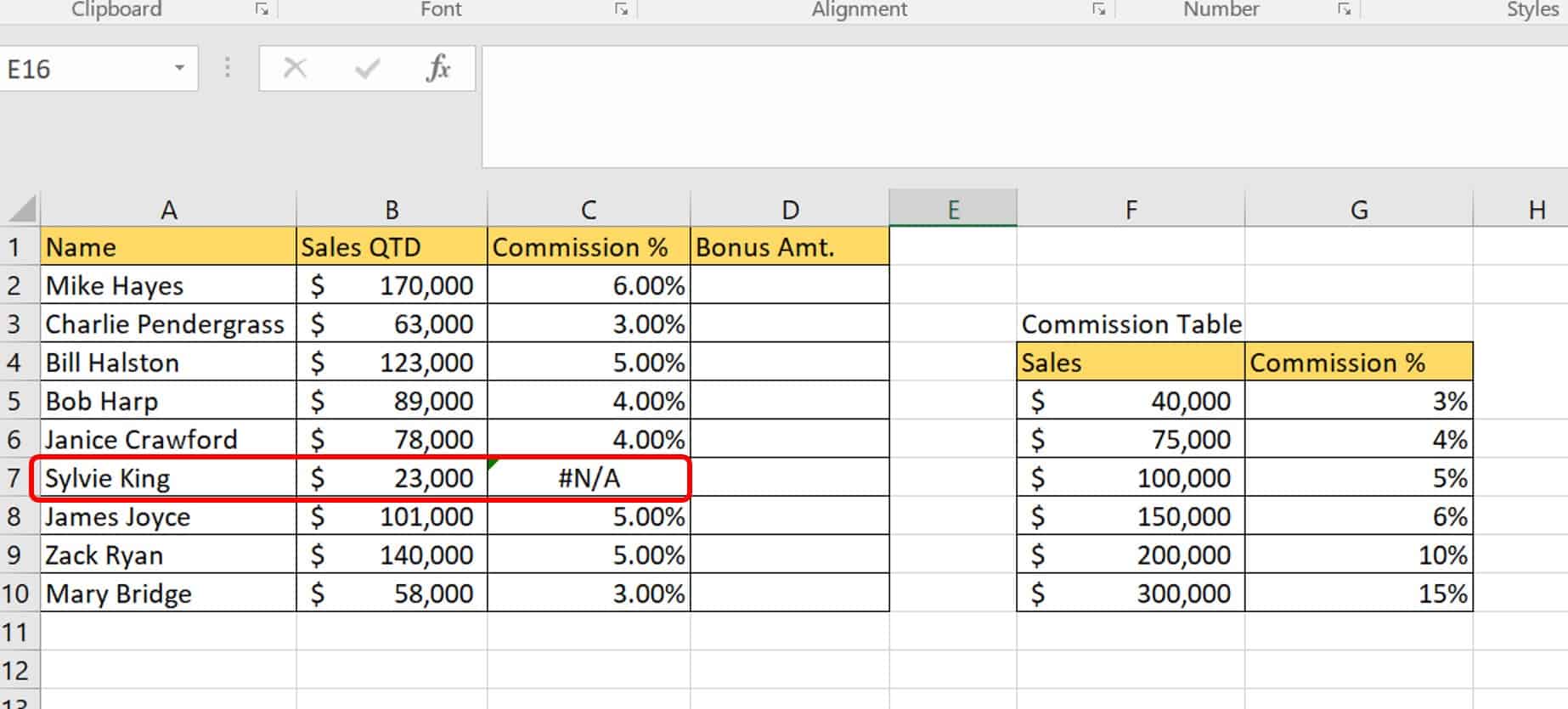
Uh-oh! As you can see from the example, you receive an #N/A error. This means the data you seek is either not where you told Excel to look or it is in the wrong format. In this case, Excel does not recognize the data present as the data it seeks because there is additional data in the cell: the choice of mate, masala, or rooibos.
To account for other data in the cell, Excel has extra characters that help out. For example, if your data table is loaded from an accounting program or other software, it may add extra spaces to each cell. Excel recognizes these extra spaces as characters and could produce the #N/A error.- Type an asterisk (*) after your drink order. The asterisk tells Excel to disregard any characters after “Chai latte”. Now, Excel returns the correct price.
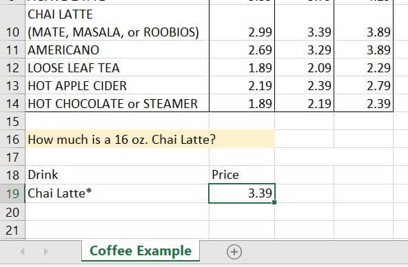
This example was an exact match VLOOKUP and returned the exact value you were seeking — not an approximation.
The fourth argument in the VLOOKUP formula, [range_lookup], is a Boolean argument, meaning that you can give it a TRUE/FALSE value or representation of a TRUE/FALSE value such as 1/0. In this formula, FALSE is an exact match, and TRUE is an approximate match.
The argument name, [range_lookup], may be misleading to many users. The approximate match does not work well with text strings and is mostly meant for strings of numbers, especially when you are looking for a value from within a range. For this type of example, you would perform an approximate match VLOOKUP.
VLOOKUP Example: How to Perform an Approximate Match
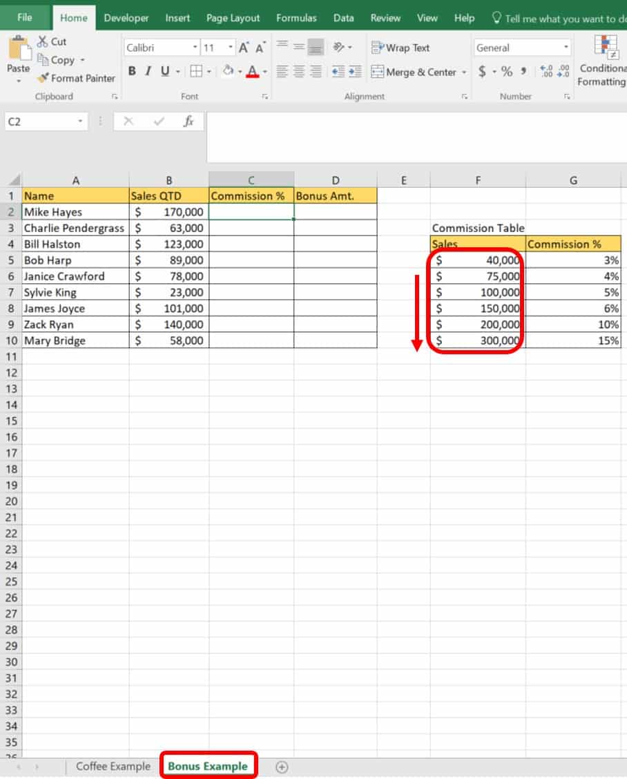
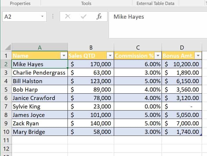
The Bonus Example worksheet in the Excel Sample Data file is an example of how to calculate sales bonuses using VLOOKUP. We added the commission table to the worksheet as a reference to show what commission percent each salesperson has earned for the quarter. Bonuses in this company start after an employee reaches $40,000 in sales and bump up percentage points as they reach each threshold. Note the sales column in the reference table is arranged in ascending order, which is important for a lookup of this type.
Follow these steps to perform an approximate match VLOOKUP in Excel.
1. Click the Bonus Example worksheet tab.
2. Click cell C2, and type =VLOOKUP( in the formula bar. This is your first VLOOKUP formula. The tool tip bar appears when you type this formula introduction.
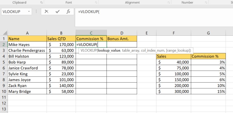
3. Type B2 (the value that Excel will use as a reference in the table, called the lookup_value) for the first argument in your VLOOKUP. It is highlighted in the same color as the argument it represents in your formula. Between each argument, type a comma (,).
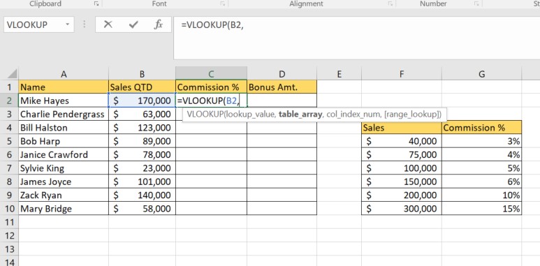
4. The second argument is table_array, which is the data table Excel uses to look up your values. You can either highlight this table manually by clicking the first cell and holding down your mouse until you have a complete selection, or you can type the range F4:G10. Type a comma (,).
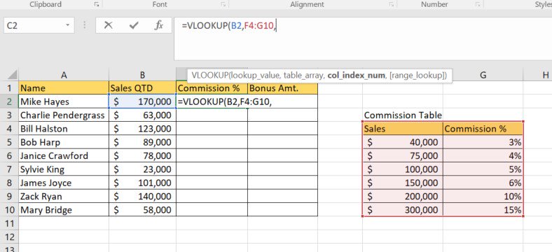
5. The third argument is col_index_num, which tells Excel the column in your data table to find the return data. Type 2 for this value. Type a comma (,).
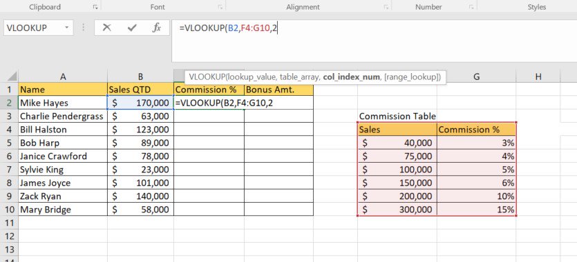
At this point, you can type a close parenthesis ) and click Enter on the keyboard or complete the formula with a fourth argument. The fourth argument automatically defaults to the approximate match, but if you want the practice, go to the next step.
6. The fourth and final argument in the approximate match VLOOKUP is [range_lookup]. If you choose to enter this argument, type TRUE or 1.

7. Type the close parenthesis ) and click Enter on the keyboard. The complete formula is =VLOOKUP(B2,F4:G10,2,1).
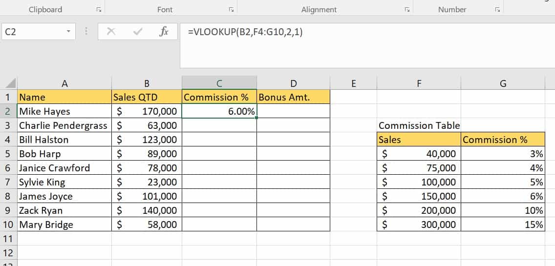
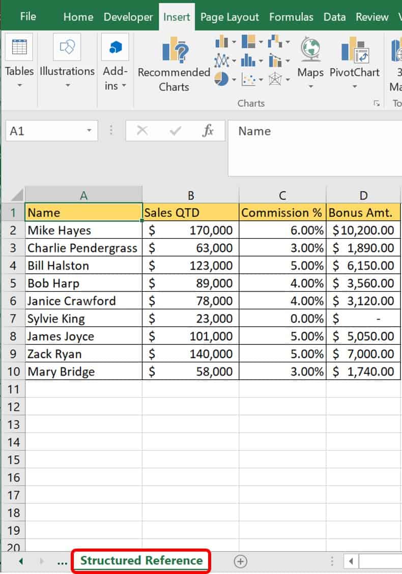
As you can see, Mike Hayes earned a 6 percent commission this quarter because he is over the threshold of $150,000 but not yet at $200,000 in sales.
8. To get the formulas into the rest of the sales team’s row, click cell C2, right-click on the mouse, and click Copy. Right-click on the mouse, click Paste Special, click Formulas (or the Paste Formula icon), and highlight cells C3 through C10 by selecting the range C3:C10. Click Enter on your keyboard.
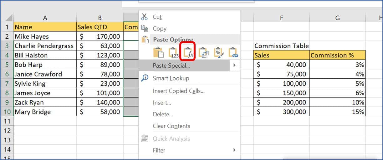
This tiles the formula down the Commission % column.
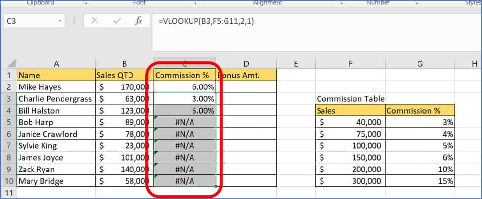
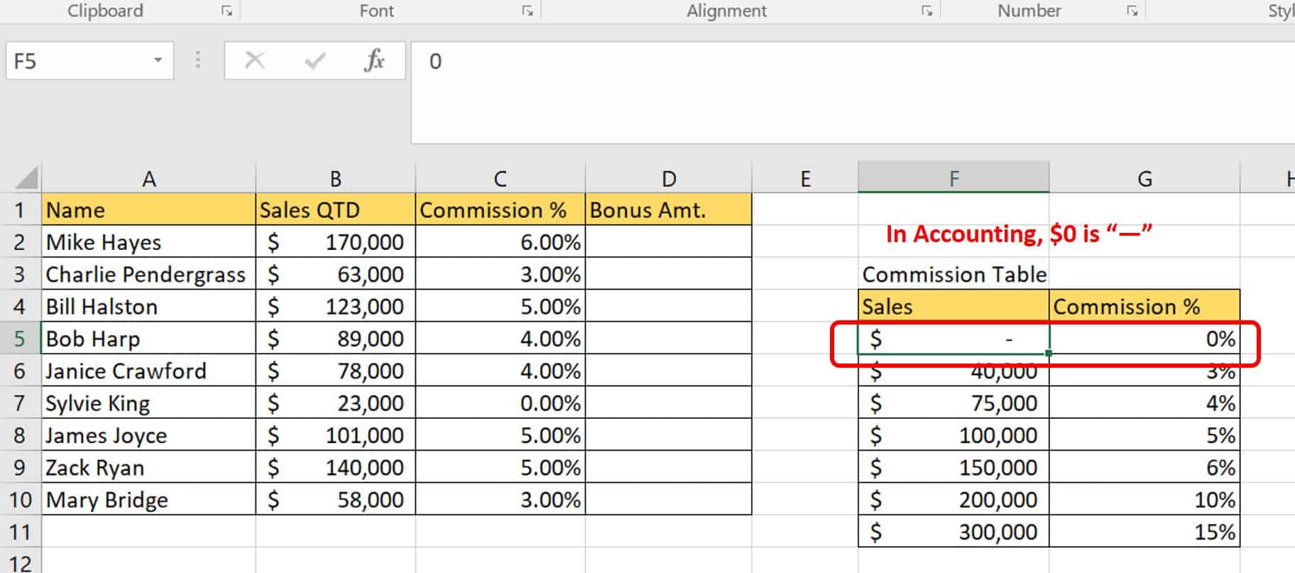
Uh-oh! Some of your formulas have an #N/A error. This occurs because tiling your formula down the Commission % column also tiles the formula down your commission data table, and Excel is looking at blank cells for your table range. To fix this, add absolute references ($) to your formula.
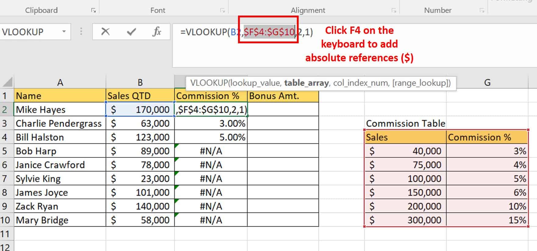
9. In your first formula in cell C2, add $ before each column and row identifier in your data table range F4:G10, so it reads $F$4:$G$10. An easy and quick way to do this is to highlight F4:G10 and click F4 on the keyboard. Click Enter on the keyboard.
10. Repeat step 8, copying C2 and pasting the rest of the column.
Uh-oh! You still have an #N/A error. However, this error is due to Sylvie King not meeting the lowest threshold eligible for a sales commission in the data table, so Excel did not find a value for $23,000 in the data table. To fix this error, you have the choice to add a lower threshold to your data table — or hope that Sylvie meets $40,000 by next quarter!
VLOOKUP uses data in a defined data table range to look vertically down a column. It specifies to Excel that the data is in a column form. A similar function is HLOOKUP, which performs a lookup in a defined data table range with the identical syntax, but it tells Excel that your data is set up in rows, or horizontally.
Many people learn the basics of VLOOKUP and HLOOKUP early in their Excel education. You may also combine the two functions when your data table is in a matrix format. In other words, your lookup values should be on the top and left side of your table. This is a two-dimensional lookup, using two pieces of information.
How to Build a Structured Reference Table
Excel data tables help you organize your data. After you build tables in Excel, they automatically resize and incorporate additional data in your formulas and keep your formulas consistent as they automatically populate. Named data tables give you an edge while building and locating formulas in large workbooks.
Follow these steps to build a structured reference table in Excel.
- Click on the Structured Reference worksheet tab in the Excel Sample Data file.
- Click the Insert tab, and click on any cell outside of the data table. Click Tables and Table, or use the Ctrl + T shortcut on the keyboard. Note: This information is already filled out in the sample data file; to create a new table follow these steps in a blank sheet.
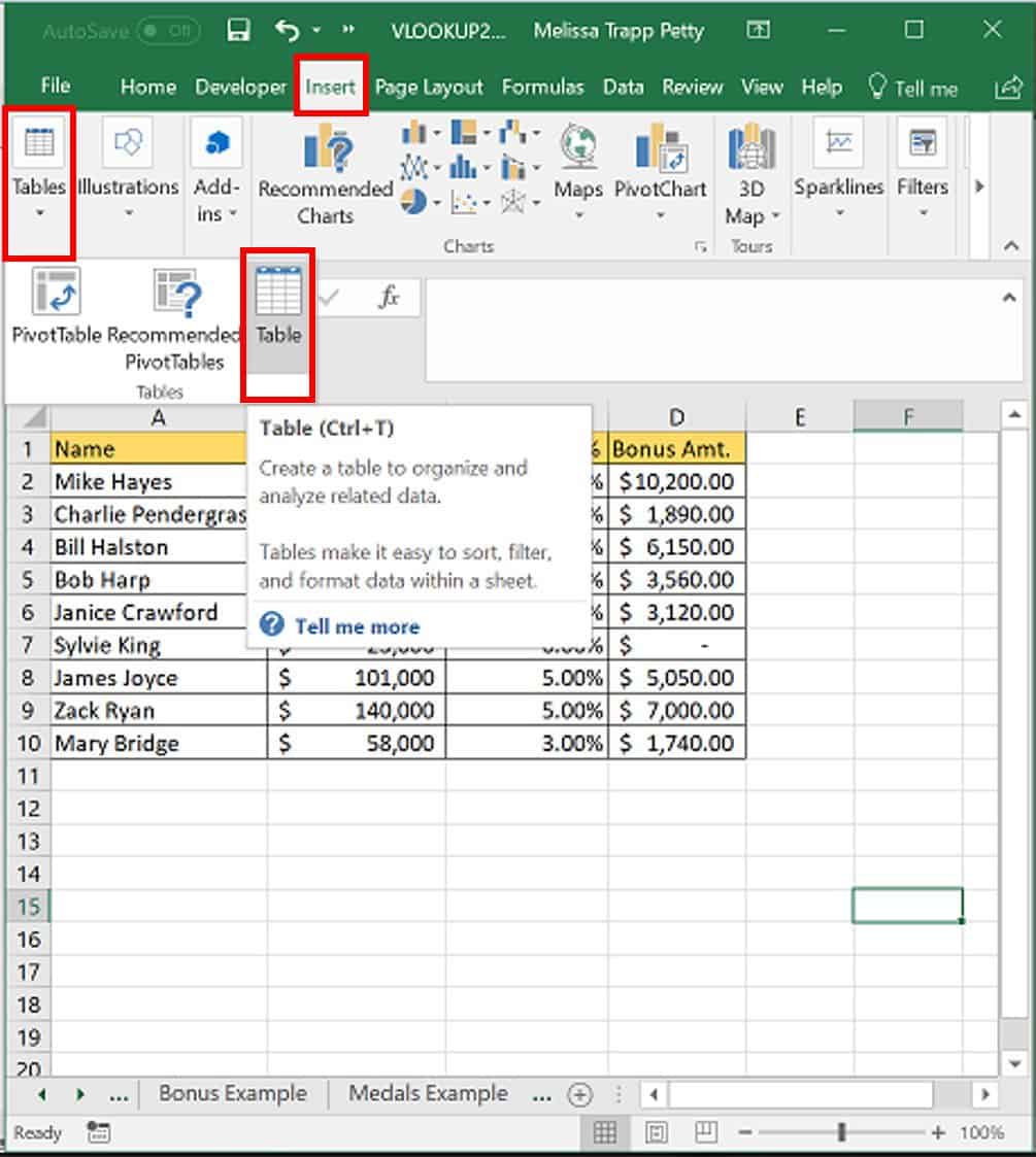
The Create Table dialogue box appears.
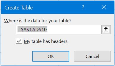
If your data table has headers, ensure that you click the My table has headers check box. Review the parameters of the table to ensure that all your data is included. Click OK. The data table autoformats with the alternate fill color.
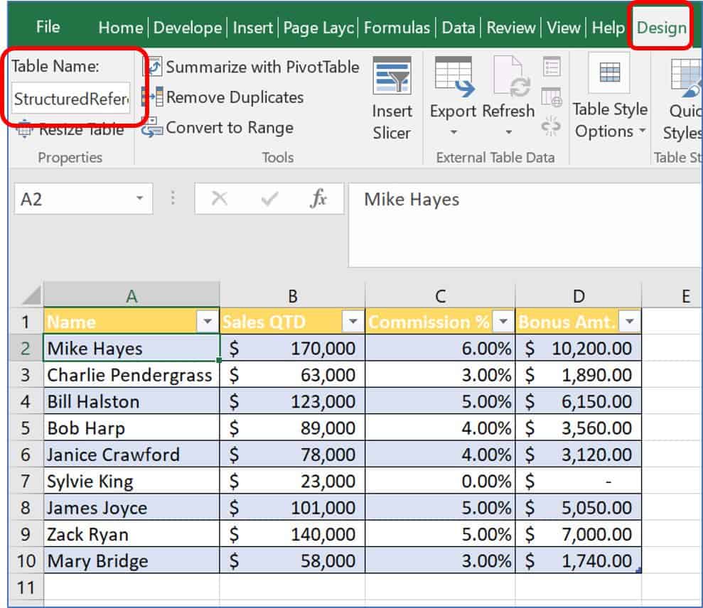
To add a table name, click the Design tab (in some versions of Excel, this will appear in the Table tab). Under Table Name, type the name StructuredReference. The name must start with either a letter or underscore (_), must not have a space or special characters, and must not conflict with an existing name in the workbook.
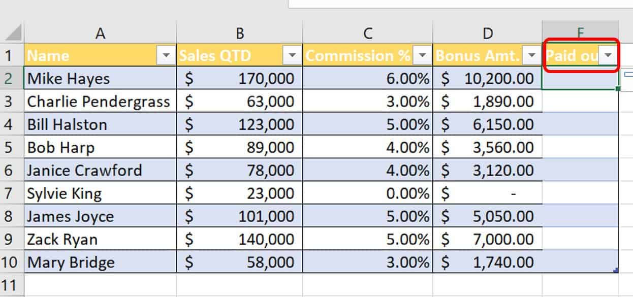
Once you name the table, you can add more headers, which are automatically formatted to match the rest of the table.
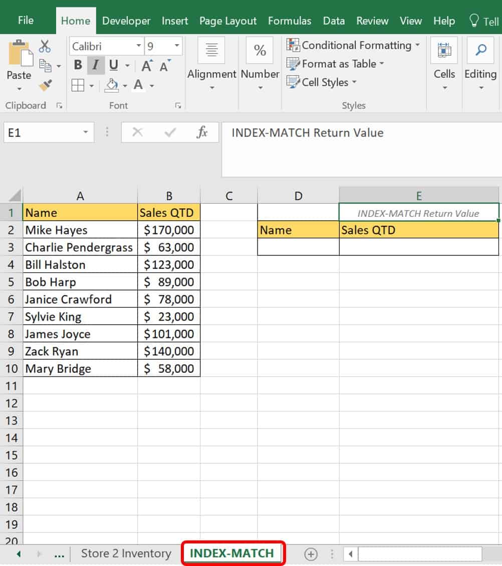
VLOOKUP Example: How to Create a Lookup Table
You can also create a lookup table, in a process similar to creating any table in Excel. Follow these steps to create a VLOOKUP table.
- Click on the Create Lookup Table worksheet tab in the Excel Sample Data file.
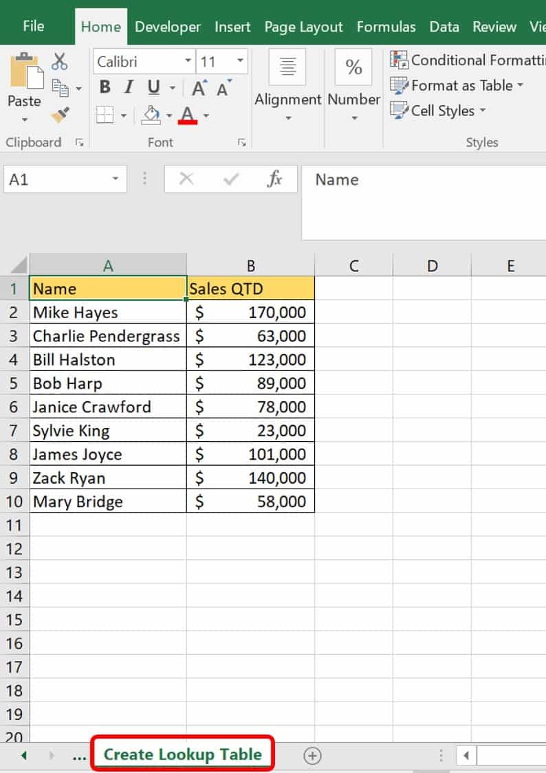
- Enter headings in the first row. This example already has two headers, Name and Sales QTD, and data entered into the table.
- Column A, the first column, has and should have the reference values. In this example, the reference values are the names of the sales staff.
- If you have other data in this worksheet, such as additional data tables, leave at least one blank row on the bottom of the table and one blank column on the right of the table. This separates the lookup table from other data.
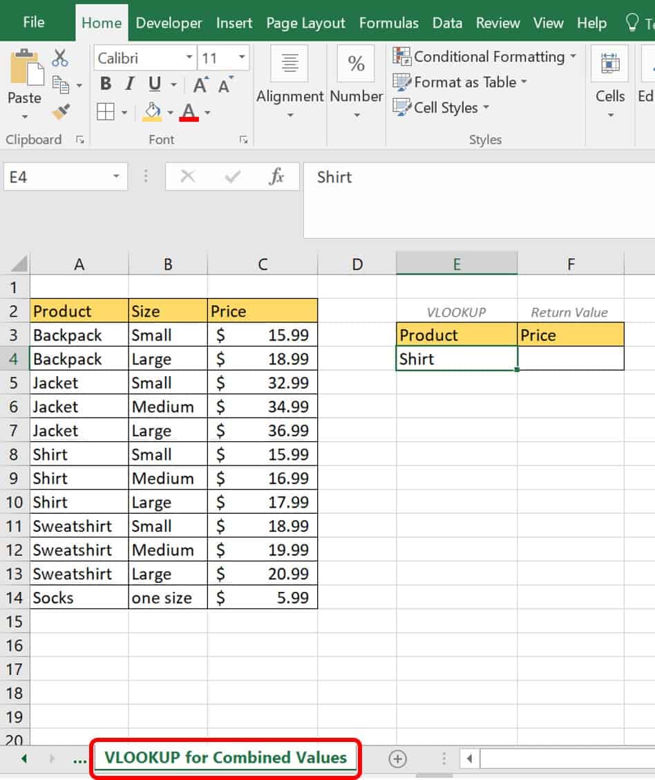
How to Create a VLOOKUP for Combined Values
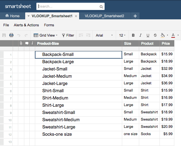
You will encounter some tables with values in the lookup column that are not unique. For example, the table below lacks a unique value for Shirt in the first column, as there are three listings. However, the second column lists three different sizes (Small, Medium, and Large). If you were to order a shirt, you would need the size to specify the price. In reality, the company that sells these products has only one record for each product and size combination.
Product | Size | Price |
|---|---|---|
Backpack | Small | $ 15.99 |
Backpack | Large | $ 18.99 |
Jacket | Small | $ 32.99 |
Jacket | Medium | $ 34.99 |
Jacket | Large | $ 36.99 |
Shirt | Small | $ 15.99 |
Shirt | Medium | $ 16.99 |
Shirt | Large | $ 17.99 |
Sweatshirt | Small | $ 18.99 |
Sweatshirt | Medium | $ 19.99 |
Sweatshirt | Large | $ 20.99 |
Socks | one size | $ 5.99 |
Follow these steps to create a VLOOKUP for combined values. The Excel Sample Data file has pre-existing data. This tutorial shows you how to turn that data into a table that Excel recognizes.
- Click the VLOOKUP for Combined Values worksheet tab in the Excel Sample Data file.
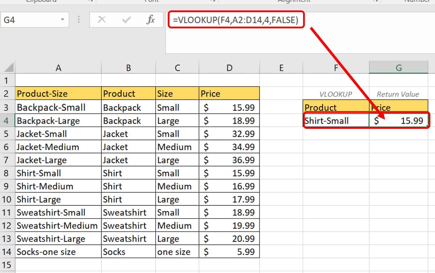
- Insert a column to the left of the Product column to create the Product-Size column, which will combine both the product and size.
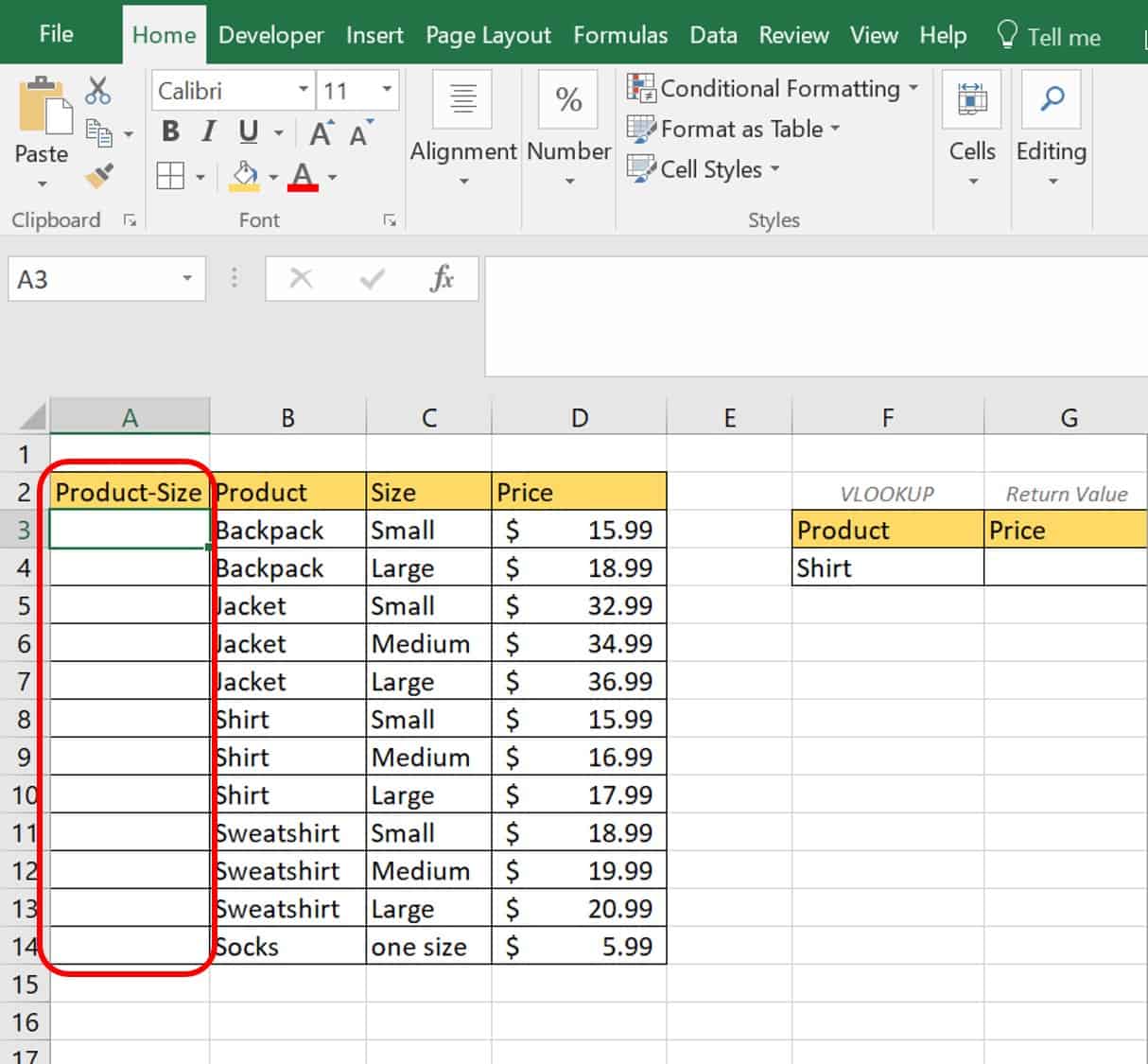
- Click on cell A3 and type =B3&”-“&C3 in the formula bar.

- Copy cell A3 and paste the formula in all the remaining cells in column A.
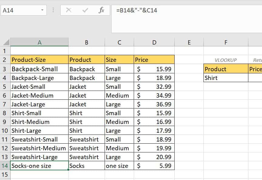
This creates a unique value for each entry in column A and allows you to type and use a VLOOKUP function for your data. The VLOOKUP formula for the price of each unique product (in this formula, we are looking for the price of a Shirt-Small) in column A is as follows:
=VLOOKUP(F4,A2:D14,4,FALSE)
To see if it works, click on any cell outside the table on the Excel Sample Data file sheet, copy the VLOOKUP formula into the formula bar, and click OK.
For a Shirt-Small, your return value is $15.99.
VLOOKUP Examples: Beginner Formulas
The following are basic concepts and examples in VLOOKUP that will work with versions of Excel 2007 and later. After you master these concepts, you can then move to more advanced material and make use of the power of VLOOKUP.
How to Do VLOOKUP from Another Worksheet
In reality, very few VLOOKUP formulas are used to look up data in the same worksheet. Most VLOOKUPs pull data from another worksheet.
Follow these steps to perform a VLOOKUP from another worksheet.
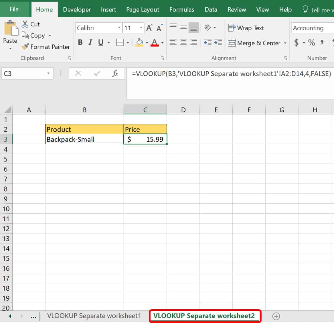
1. Click on the VLOOKUP Separate worksheet1 worksheet tab.
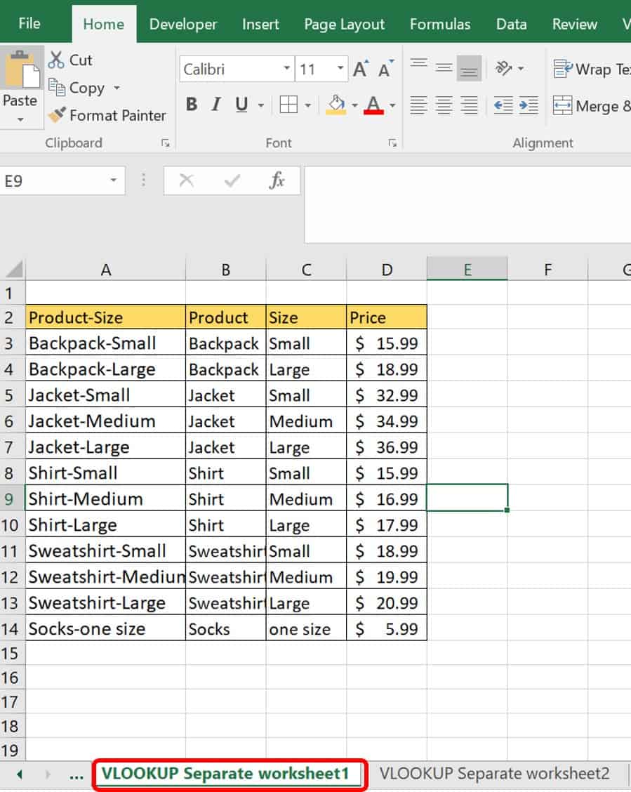
This data table has the product list downloaded from an accounting program.
2. Click on VLOOKUP Separate worksheet2 worksheet tab.

This worksheet has the lookup box. You will draw from the VLOOKUP Separate worksheet1 as the data table to populate this worksheet’s lookup box.
3. Click on cell C4 in VLOOKUP Separate worksheet2, and type the following formula:
=VLOOKUP(B3,'VLOOKUP Separate worksheet1'!A2:D14,4,FALSE)
Let’s break down this formula:
Argument | Value | Meaning |
|---|---|---|
Lookup_Value | B3 | The vertical lookup reference |
When you get to the second argument, table_array, you are pulling data from the first worksheet, VLOOKUP Separate worksheet1. To do so, you must tell Excel that your data is on another worksheet, and for the syntax, you’ll start with the name of the worksheet surrounded by single quotation marks (‘), followed by an exclamation point (!), then the cell range:
Argument | Value | Meaning |
|---|---|---|
Table_array |
| The range of cells Excel looks through to find the lookup reference in the table |
You can also manually go to the other worksheet and designate the table_array by selecting the range of cells. Excel will automatically recognize that you are on another worksheet and add the correct syntax.
The last two arguments are the same as you’ll usually find in a VLOOKUP. In this case, they are:
Argument | Value | Meaning |
|---|---|---|
Col_index_num | 4 | The column number where the return data is located |
[range_lookup] | FALSE | The exact value |
4. Click Enter on the keyboard.
How to Do VLOOKUP from a Different Workbook
You will also commonly do a VLOOKUP from another workbook.
Follow these steps to execute a VLOOKUP from another workbook:
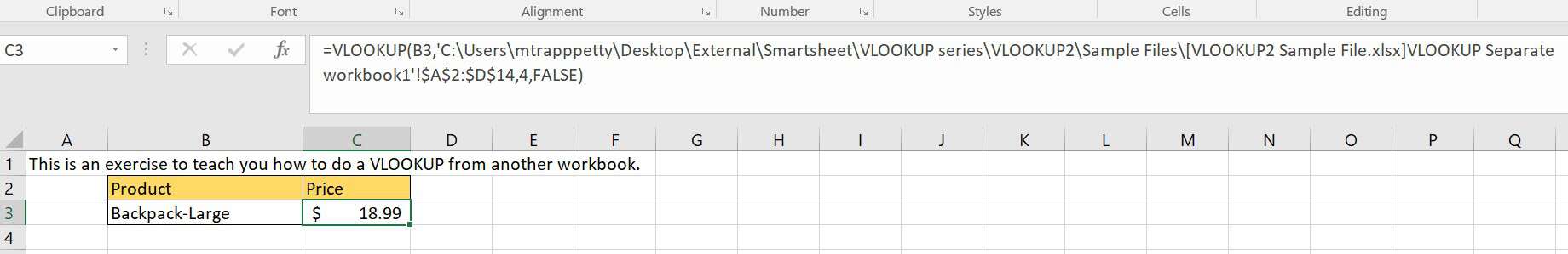
1. Click on the VLOOKUP Separate workbook1 worksheet tab in the VLOOKUP2.2 Sample File Excel file that you can download here .
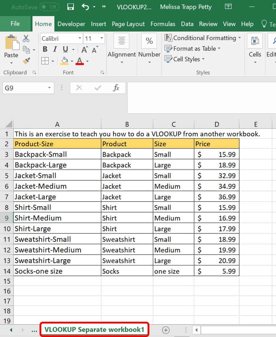
As source data, this worksheet has product data for a clothing manufacturer.
2. Open the VLOOKUP2.2 Excel file. There is only one worksheet tab: VLOOKUP Separate workbook2. For this function, both workbooks should be open while you are writing the formula. After the formula has been written, the source workbook does not need to be open. Excel will update its location after you close it in the formula.
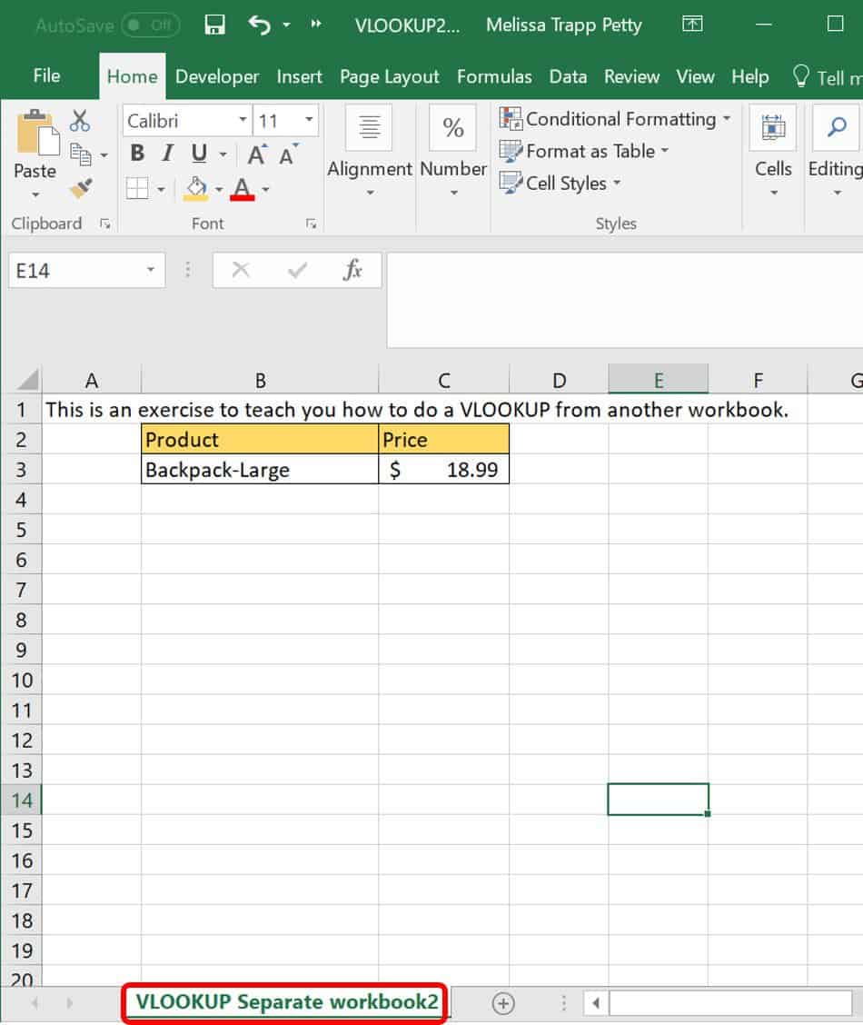
This worksheet has the reference data and the lookup box, and it draws data for the VLOOKUP from the first workbook and worksheet.
3. In cell C3 of the VLOOKUP Separate workbook2 of VLOOKUP2.2 workbook, type the following formula:
=VLOOKUP(B3,'[VLOOKUP2 Sample File.xlsx]VLOOKUP Separate workbook1'!$A$2:$D$14,4,FALSE)
Let’s break down this formula:
Argument | Value | Meaning |
|---|---|---|
Lookup_Value | B3 | The vertical lookup reference |
When you get to the second argument, table_array, you are looking to pull data from the first workbook, VLOOKUP Separate workbook1. To do so, you must tell Excel that your data is on another worksheet and in another workbook. For the syntax, you’ll add the name of the workbook in brackets [], then the name of the worksheet with an exclamation point (!) before the cell range. Both the workbook name and the worksheet name are surrounded by single quotations (‘):
Argument | Value | Meaning |
|---|---|---|
Table_array | '[VLOOKUP2 Sample File.xlsx]VLOOKUP Separate workbook1'!$A$2:$D$14 | The range of cells Excel looks through to find the lookup reference in the table |
You can also manually go to the other workbook and designate the table_array by selecting the range of cells for the lookup. Excel will automatically recognize that you are on another workbook and add the correct syntax. When you close the lookup table workbook, your VLOOKUP formula will still work, but it will display the full path for the lookup workbook, as shown below:
The last two arguments are the same as you’ll usually find in a VLOOKUP. In this case, they are:
Argument | Value | Meaning |
|---|---|---|
Col_index_num | 4 | The column number where the return data is located |
[range_lookup] | FALSE | The exact value |
4. Click Enter on the keyboard.
VLOOKUP Example: Combining Data Sets
If you want to combine data sets, a piece of data must anchor them both. In other words, both sets of data should have at least one piece of data in common, so they can cross from one table to the other.
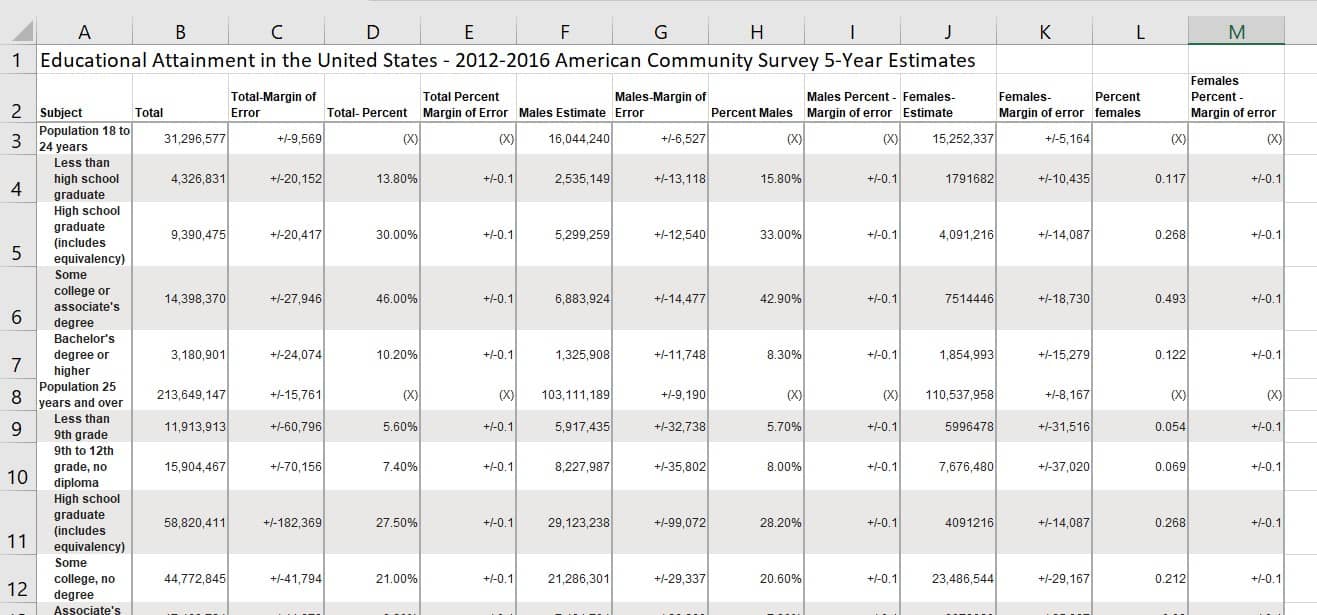
The following example includes data from the American Community Survey (ACS) on educational attainment in the United States. Age and education levels stratify the data. There are two separate tables, downloaded separately from ACS: one for males and one for females. Since ACS stratifies its data the same way, it is possible to combine these Excel tables to further organize it for your reporting needs.
Excel can help do this with a VLOOKUP, but only because both data sets have a common column. Even if the order of the column was sorted differently, it would not matter, because the data is still present in the first row for each table.
How to Combine Data Sets in Excel
Follow these steps to combine data sets in Excel.
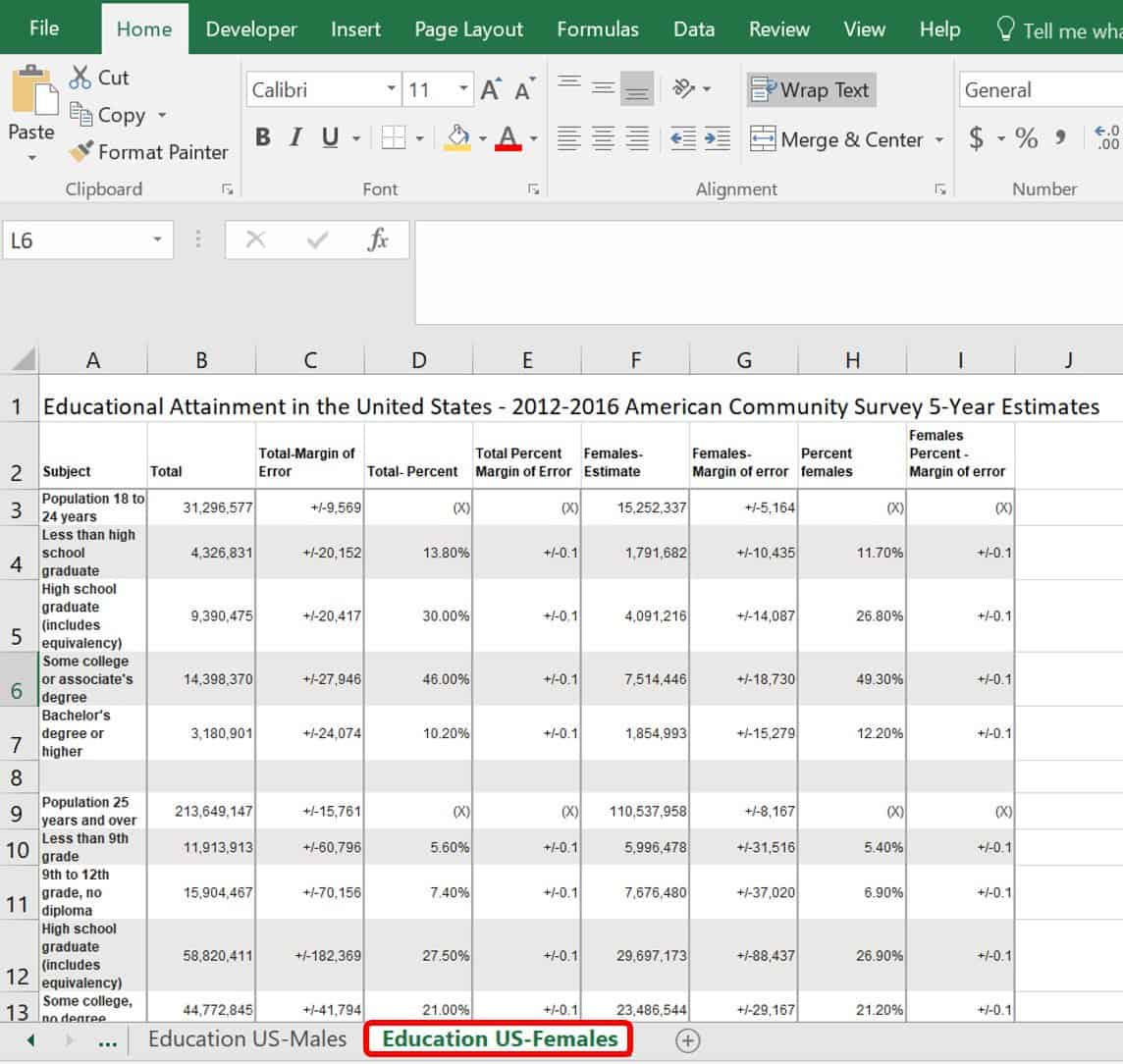
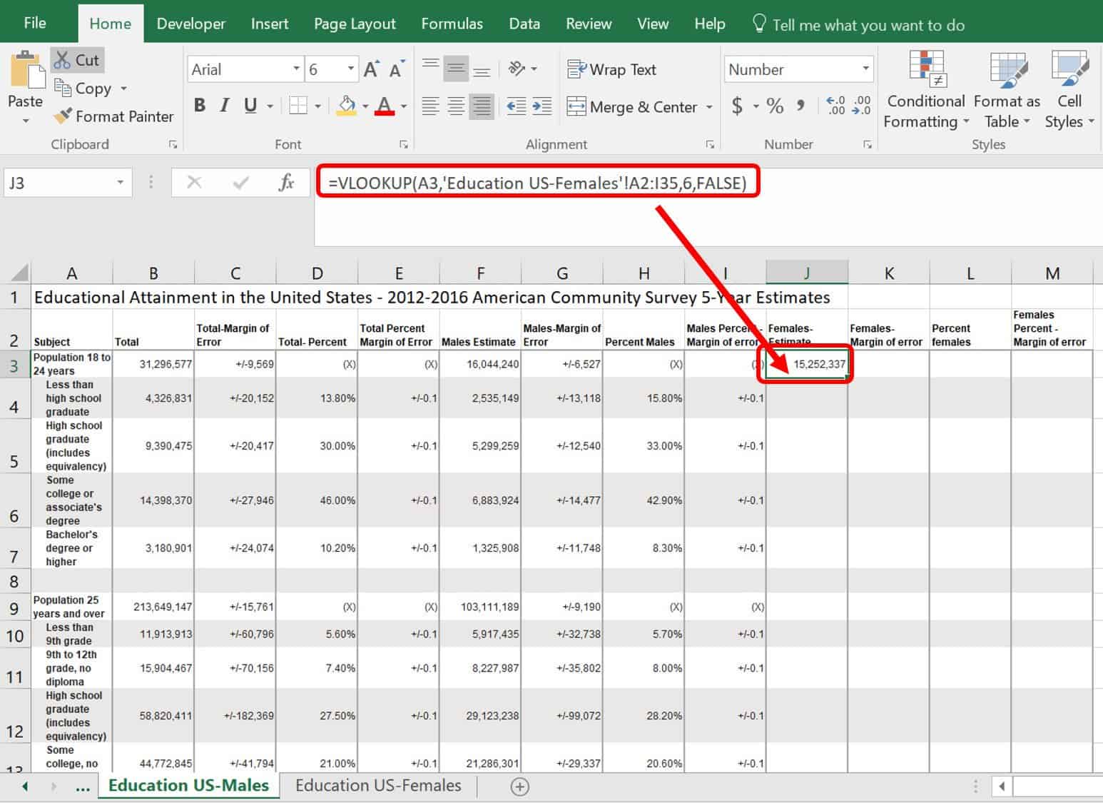
1. For this exercise, there are two worksheet tabs, Education US-Males and Education US-Females, in the Excel Sample Data file. Note: On Education US-Males, we added extra column headers so that you can include data from the Education US-Females worksheet. Again, the data on the second sheet does not have to be ordered in the same way if the row headers are present on both sheets in the first column.
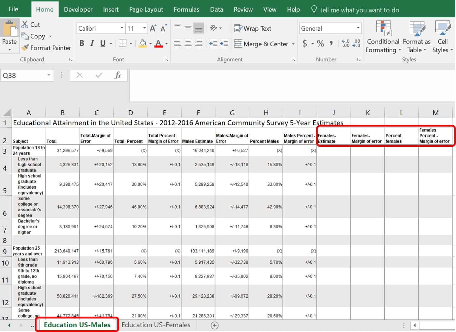
2. On the Education US-Males worksheet, click on cell J3 and type the following formula:
=VLOOKUP(A3,'Education US-Females'!A2:I35,6,FALSE)
Here’s the breakdown of the formula:
Argument | Value | Meaning |
|---|---|---|
Lookup_Value | A3 | The vertical lookup reference |
Table_array | 'Education US-Females'!A2:I35 | The range of cells Excel looks through to find the lookup reference in the table |
Col_index_num | 6 | The column number with the required data |
[range_lookup] | FALSE | The exact value defined |
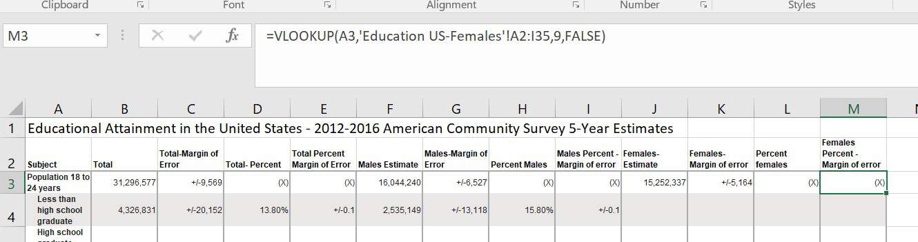
This formula matches the Females Estimate column in the Education US-Females worksheet, which is column 6 in the Education US-Males worksheet. You also need columns 7, 8, and 9. The formulas for loading these into your new table are exactly the same, except for the column numbers in argument three.
3. In cells K3, L3, and M3 Education US-Males worksheet, type the following formulas, respectively:
K3=VLOOKUP(A3,'Education US-Females'!A2:I35,7,FALSE)
L3=VLOOKUP(A3,'Education US-Females'!A2:I35,8,FALSE)
M3=VLOOKUP(A3,'Education US-Females'!A2:I35,9,FALSE)
As you can see, the underlined numbers are the only changes to the formula, and they refer to the column number where the data is drawn.
4. To keep the data consistent for the next step, you must add absolute references to the data table (table_array). To do so, click on your first formula in cell J3, and select and highlight the third argument, 'Education US-Females'!A2:I35. On the keyboard, click the F4 key. One click adds the absolute reference ($) in the correct place. Click Enter on the keyboard.
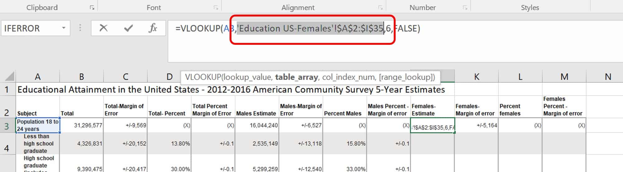
5. Perform step 4 for cells K3, L3, and M3. Now your cells have absolute references built in, and you can apply their formula to the remainder of your data table.
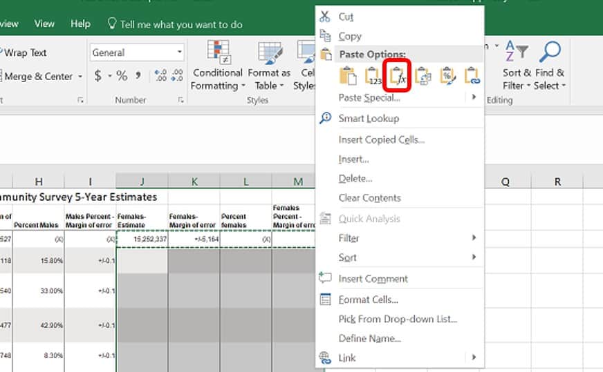
6. Select and copy cells J3 through M3.
7. Paste these cell formulas into the other rows of your table using either the Ctrl + V shortcut or by right-clicking on the mouse and clicking Paste Formulas. With the latter method, you keep the formatting intact.
At this point, your table is complete. You can play with the table and titles, ensuring that they are accurate for your needs. You can also turn the whole data table into an Excel “table” for future use.
VLOOKUP Formulas with Wildcard Characters
In VLOOKUP formulas, you can use wildcard characters to help look up values or spellings you are unsure of:
- Use a question mark (?) to match any single character.
- Use an asterisk (*) to match any sequence of characters.
How to Use Wildcard Characters in VLOOKUP
Follow these steps to use wildcard characters in VLOOKUP.
1. Click on the Wildcards tab in the Excel Sample Data file.
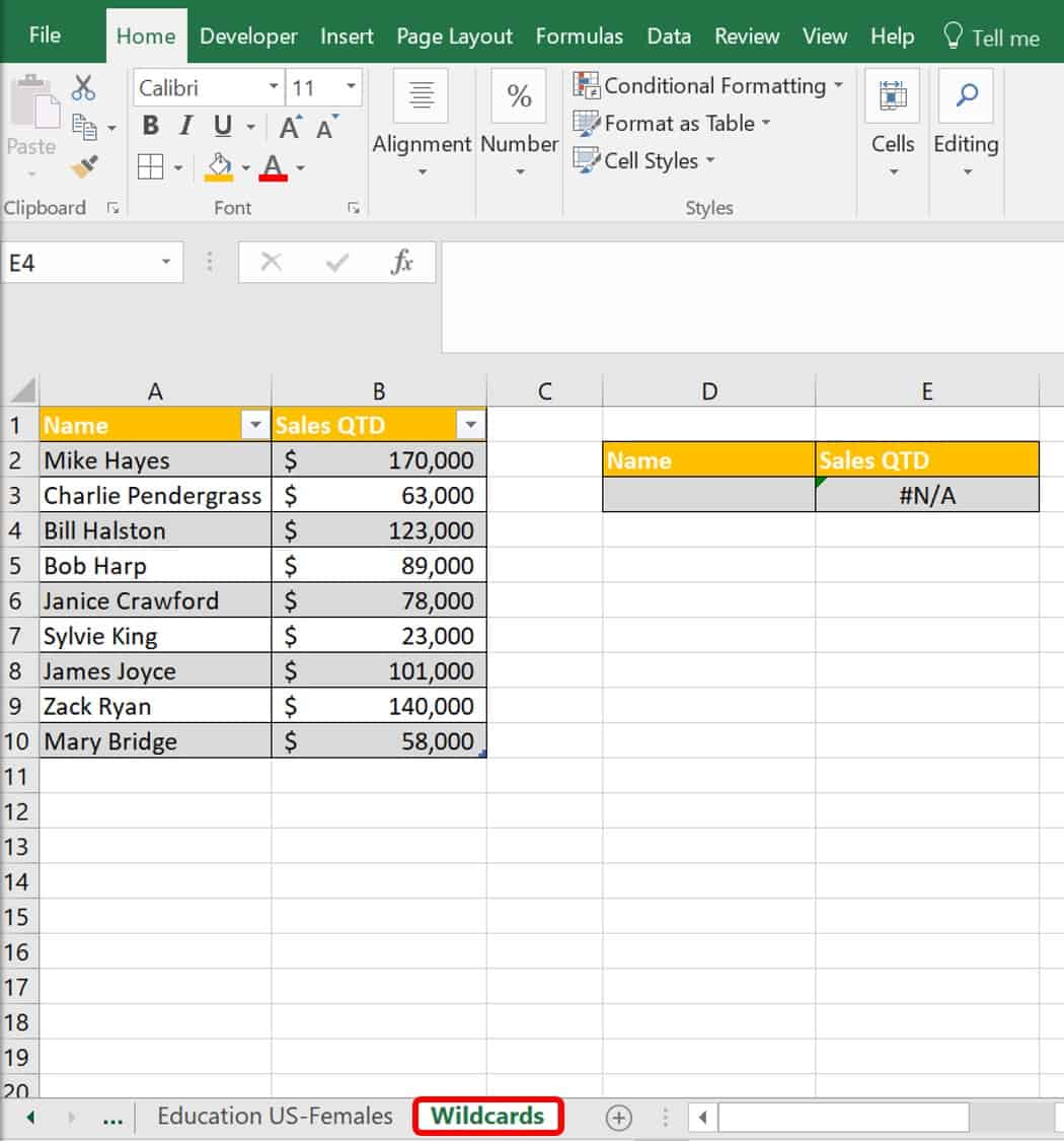
This worksheet has a table of sales team members and their quarter-to-date (QTD) sales. There is a Sales QTD lookup box based on the salesperson’s name. Wildcard characters can help in the following scenarios:
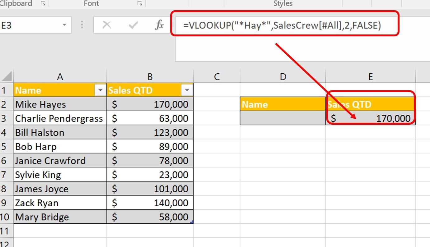
Look up the salesperson’s name starting or ending with certain characters. In this scenario, you are not sure of the exact spelling of Mike Hayes’ name. You can click cell D4 (Name lookup box) and type Mike H*. Excel recognizes that the asterisk (*) stands for several missing letters.
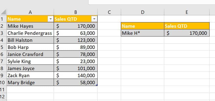
You could also add the asterisk to the beginning of Mike’s name to yield the same result or use several asterisks to replace letters you are unsure of.
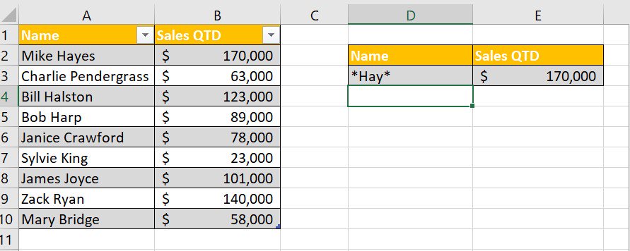
You could also add the wildcard to your VLOOKUP formula. For example, instead of entering your salesperson’s name in cell D3, you could add what you know into the VLOOKUP formula.
Troubleshooting the VLOOKUP Formula
Excel compares your reference value (lookup_value) with the data in the table and matches it, before scanning to your return value. If the value is not present, you will receive an #N/A error. However, even if your value is present in the table, there are still three possible reasons you could get an error:
- A Mismatch in Format: Either your reference value or the table data is formatted as a number and the other is formatted as text. You can fix this error by reformatting so that they match.
- Extra Spaces: Your reference or your table data has leading, lagging, or embedded spaces. To check for extra spaces in a cell, use the LEN function, which returns the number of characters in a cell. To correct for excess leading or lagging spaces, use the TRIM function.
- Other Characters: If the TRIM function does not solve your problem, you could still have other characters in either the reference or data table. Functions that help solve this problem include SUBSTITUTE or CLEAN, or you can add macros. Use SUBSTITUTE to change from characters like the forward slash to blank spaces or empty strings. Use CLEAN to remove nonprinting characters.
Problems When Sorting the VLOOKUP Formula
Initially, your VLOOKUP may return the correct results. But sometimes you may start seeing incorrect results after you sort the data table. This problem is not unique to VLOOKUP, as it can be found in other lookup functions such as INDEX-MATCH and HLOOKUP. To fix this problem, review your formulas and ensure that they are referencing the correct worksheet. This is an Excel bug that is easy to fix.
Excel 2013 introduced the FORMULATEXT function. Adding FORMULATEXT to the side of your cells enables you to see the formulas in their entirety and to check for errors.

The formulas for the data table are in column C.
- Click on a cell in row E or F (you can use any cell that doesn’t already have data).
- Type =FORMULATEXT and then click on the cell with the formula you want to see.
Now you can take a closer look at the formula and see what needs to be changed without affecting the original cell.
Excel VLOOKUP: Tips, Rules, and Troubleshooting
This review of the Excel VLOOKUP basics will help you build up to the intermediate material in the next sections. Some details to remember:
- You can sort your tables in any way, but your left column should not have duplicate values.
- Use absolute cell references ($) in your table_array argument to ensure that you can copy and paste your formula to other cells.
- Click F4 to add absolute references to your table_array.
- VLOOKUP formulas read from left to right.
- In approximate match lookups, make sure your lookup value is larger than the smallest value you have identified. Otherwise, you will return an #N/A error.
- In approximate match lookups, always sort the data in ascending order in the data table (table_array).
- Values in VLOOKUP formulas are not case-sensitive, so you do not have to worry about uppercase or lowercase when typing formulas.
- Your col_index_num cannot be less than one (1). One signifies the first column.
- VLOOKUP can only look to the right in its search.
- The last argument, [range_lookup], is automatically set to TRUE (approximate match), unless you specify it as FALSE (exact match).
- The VLOOKUP formula works the same in all versions of Microsoft Excel.
- The #N/A error means that Excel cannot find the value you are seeking.
- The table data you are searching for may be on the same worksheet, on a different worksheet, and even in a different workbook.
VLOOKUP Examples: Intermediate Formulas
As you gain more experience with VLOOKUP, you will want to perform more complex functions. Before you move on, review the basic syntax and usage of VLOOKUP by reading this article.
How to Combine VLOOKUP and HLOOKUP Functions
Follow these steps to combine VLOOKUP and HLOOKUP functions.
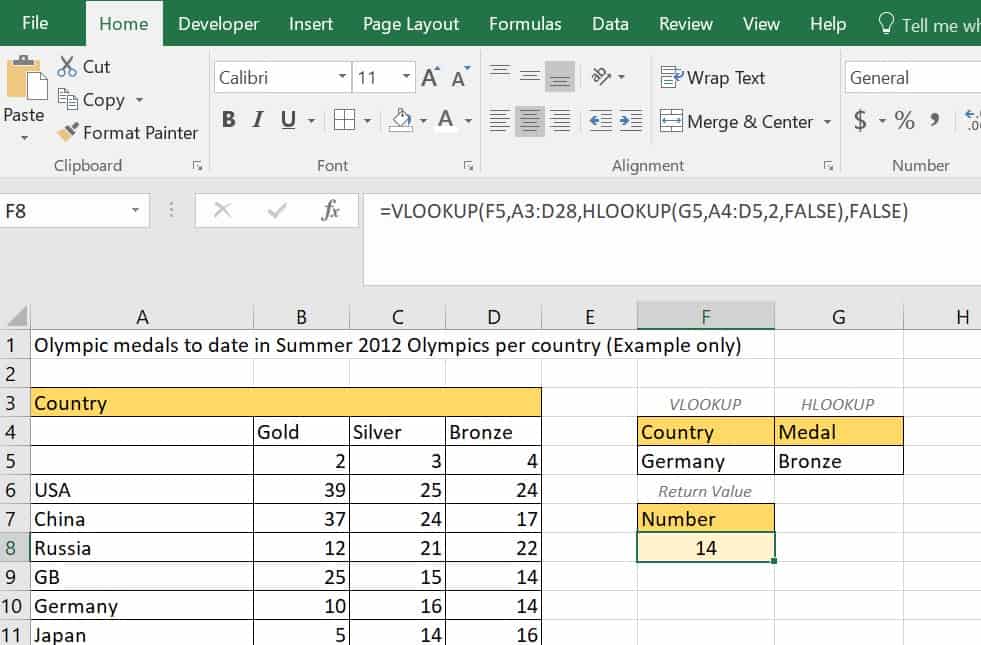
1. Click the Medals Example worksheet tab in the Excel Data Sample File.
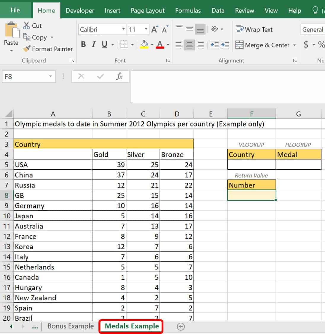
This worksheet has a matrix of data with headers in both the row across the top and the column along the left. This is a fictitious table of gold, silver, and bronze medals earned in the 2012 Summer Olympics by each country. To the right side of the data table are both VLOOKUP and HLOOKUP boxes to enter the country and type of medal. Type the VLOOKUP with a nested HLOOKUP formula in the return value box (F8).
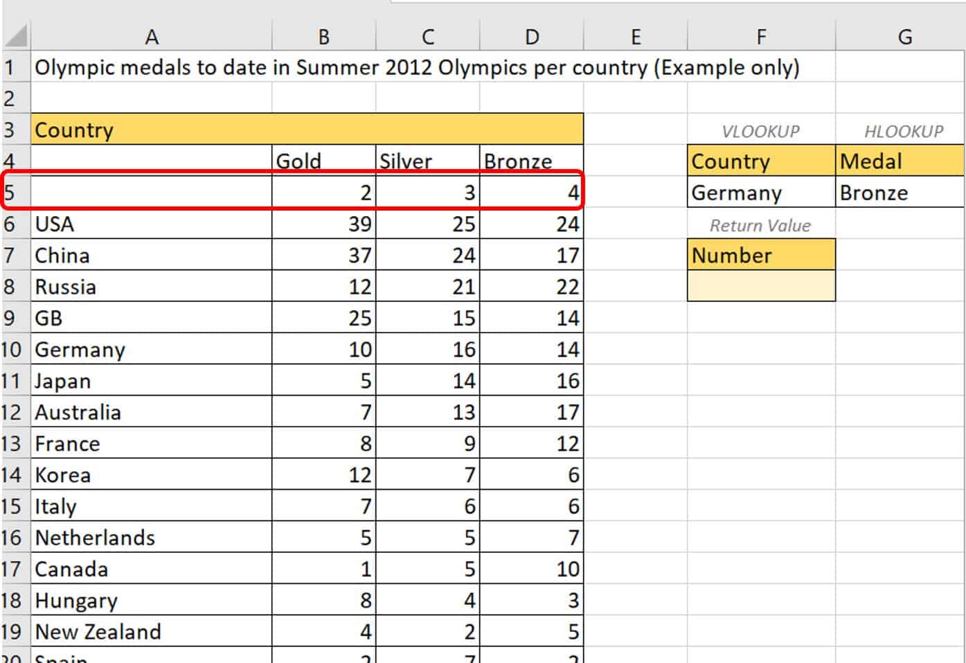
2. In the vertical lookup box, type Germany, and in the horizontal lookup box, type Bronze. This gives you values to follow in this example.
3. Insert a blank row above row 5. Since VLOOKUP is only capable of referring to a number in the col_index_num, type numbers 2, 3, and 4 in cells B5, C5, and D5, respectively.
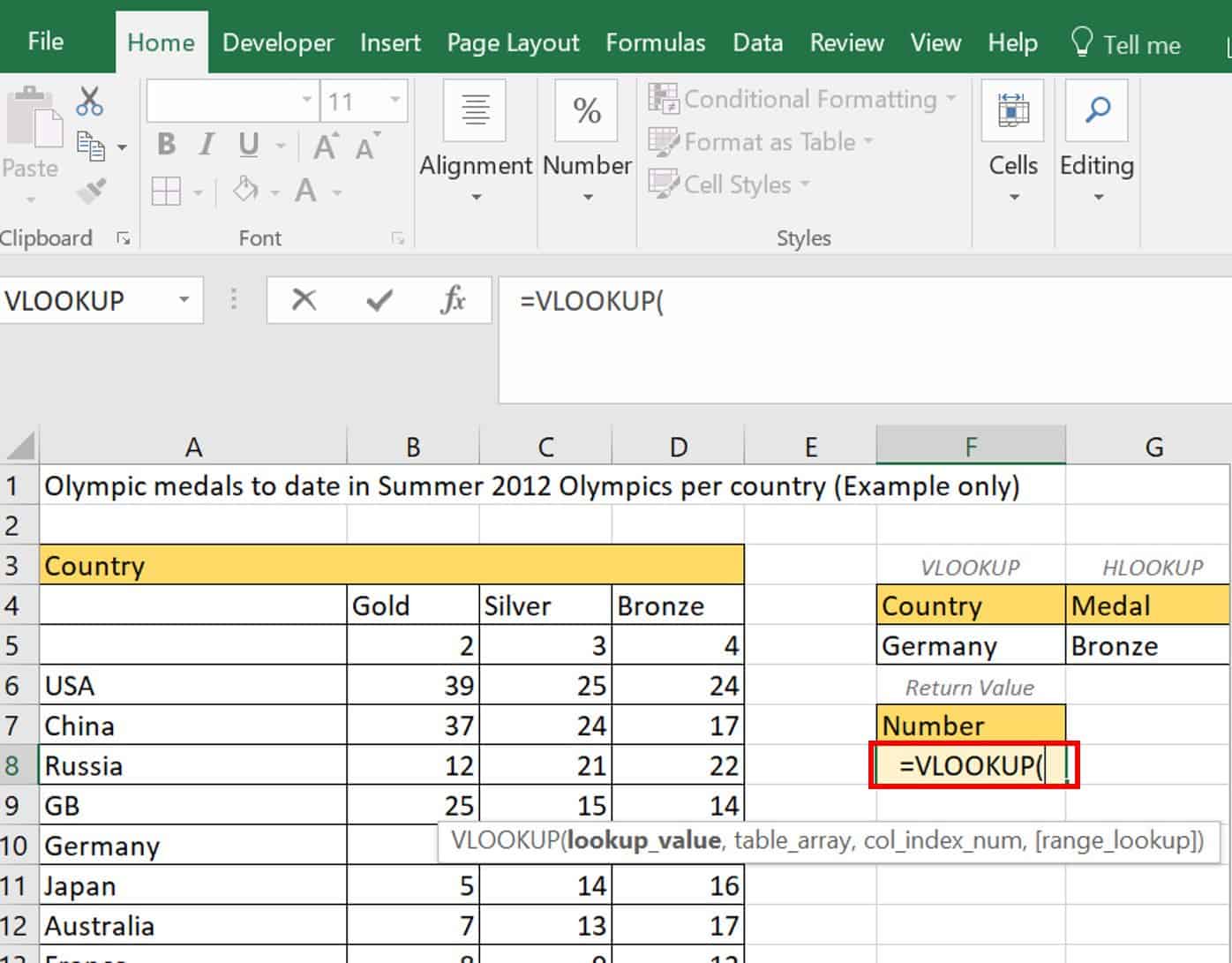
Type =VLOOKUP( in cell F8 to signal to Excel that you are starting a VLOOKUP function.
4. As with the earlier VLOOKUP formula example, add the first two arguments separated by commas below:
Argument | Value | Meaning |
|---|---|---|
Lookup_value | F5 | Vertical lookup reference |
Table_array | A3:D28 | Data table parameters |
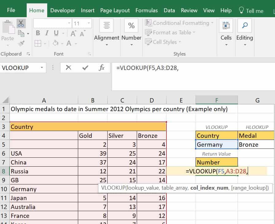
So far, your formula is =VLOOKUP(F5,A3:D28.
5. Add the second function in the third argument, col_index_num. Instead of inserting a column number, add HLOOKUP as a nested function in a new set of parentheses, like a formula within a formula. Type HLOOKUP( to signal to Excel that you are starting another function.
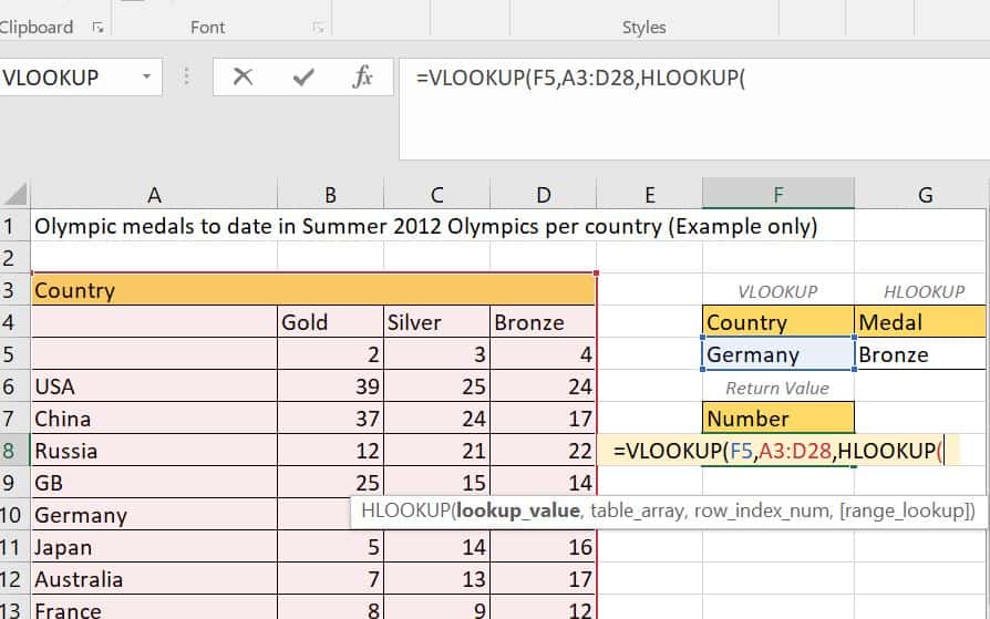
6. Add the four HLOOKUP functions:
Argument | Value | Meaning |
|---|---|---|
Lookup_value | F5 | Vertical lookup reference |
Table_array | A4:D5 | Row parameters in the data table |
Row_index_num | 2 | The row where the return value is located |
[range_lookup] | FALSE | An exact value |
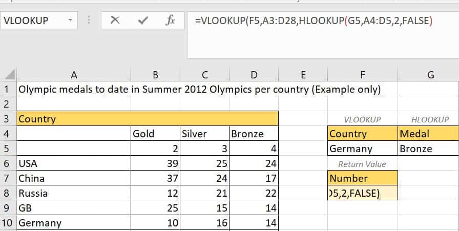
7. Add the last VLOOKUP argument, FALSE.
8. Click Enter on the keyboard.
How to Combine VLOOKUP with MATCH
Combining the VLOOKUP and MATCH functions enables you to construct a flexible lookup formula that is easier to copy across a worksheet. The MATCH formula replaces col_index_num in the VLOOKUP formula. This combination also helps prevent problems when you add new columns to the lookup table or if you rearrange the columns. This scenario is similar to using a VLOOKUP-HLOOKUP combination, except you do not need a proxy number for your row.
Follow these steps to perform a VLOOKUP-MATCH.
1. Click the VLOOKUP-MATCH Example worksheet tab.
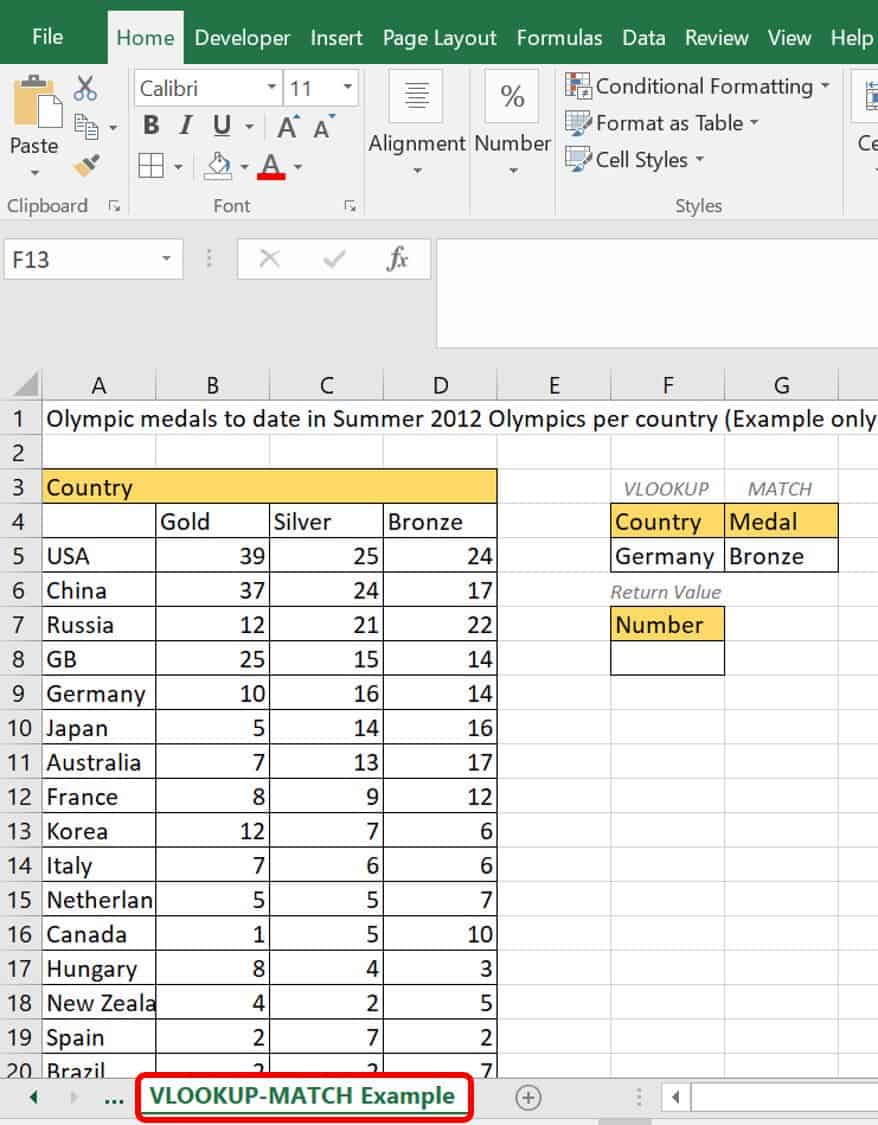
This worksheet has a data table that is a matrix with headers in both the top row and the first column. There are VLOOKUP and MATCH boxes to help you visualize where the formula draws its data. The return value box (F8) is where you will type the VLOOKUP with the nested MATCH formula.
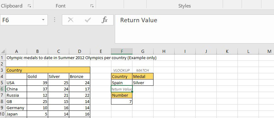
2. Notice Germany in the VLOOKUP box and Bronze in the MATCH lookup box. This provides values to follow along with in this example.
3. Like the VLOOKUP-HLOOKUP combination, VLOOKUP-MATCH replaces the third argument (col_index_num) in the VLOOKUP formula. This is a nested MATCH function. The overall formula in cell F8 will be:
=VLOOKUP(F5,A4:D28,(MATCH(G5,A4:D4,0)),FALSE)
Excel performs the internal function (MATCH) first, then the VLOOKUP function.
The MATCH formula nested in the overall formula is:
Argument | Value | Meaning |
|---|---|---|
Lookup_Value | G5 | The lookup reference |
Lookup_Array | A4:D4 | The range of cells Excel looks through to find the lookup reference in the table |
Match type | 0 | The first value exactly equal to the lookup value |
Place this formula (nested) inside the VLOOKUP formula, replacing the third argument. The VLOOKUP formula is:
Argument | Value | Meaning |
|---|---|---|
Lookup_Value | F5 | The vertical lookup reference |
Table_array | A4:D28 | The range of cells Excel looks through to find the lookup reference in the table |
Col_index_num | MATCH formula | The MATCH value that defines the column number |
[range_lookup] | FALSE | The exact value |
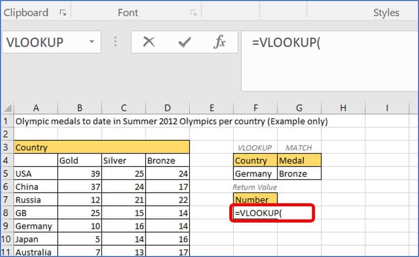
4. Click cell F8 and type =VLOOKUP(.
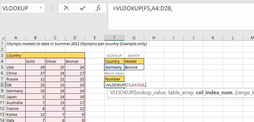
5. Type the first two arguments in the VLOOKUP formula, F5 and A4:D28, separated by a comma.
6. Type the MATCH formula, (MATCH(G5,A4:D4,0)), as the third argument in the VLOOKUP function.
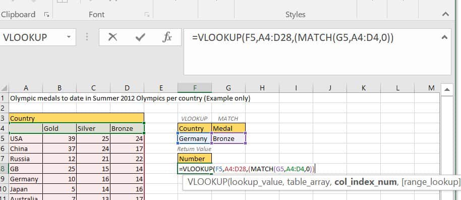
7. Type a comma (,) and the last VLOOKUP argument, FALSE. Close the combined function with a parenthesis ). Click Enter on the keyboard.
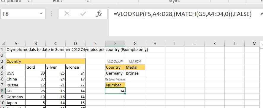
As you can see, in this data table, Germany won 14 bronze medals. If you change both the values in the VLOOKUP and MATCH boxes, you consistently get the correct return value from the data table.
How to Combine IF and VLOOKUP Functions
When you add the IF function to the VLOOKUP, the cell remains blank instead of showing an error if your VLOOKUP does not have a value to return.
Follow these steps to add an IF function to your VLOOKUP.
1. Click on the VLOOKUP-IF Example sample file.
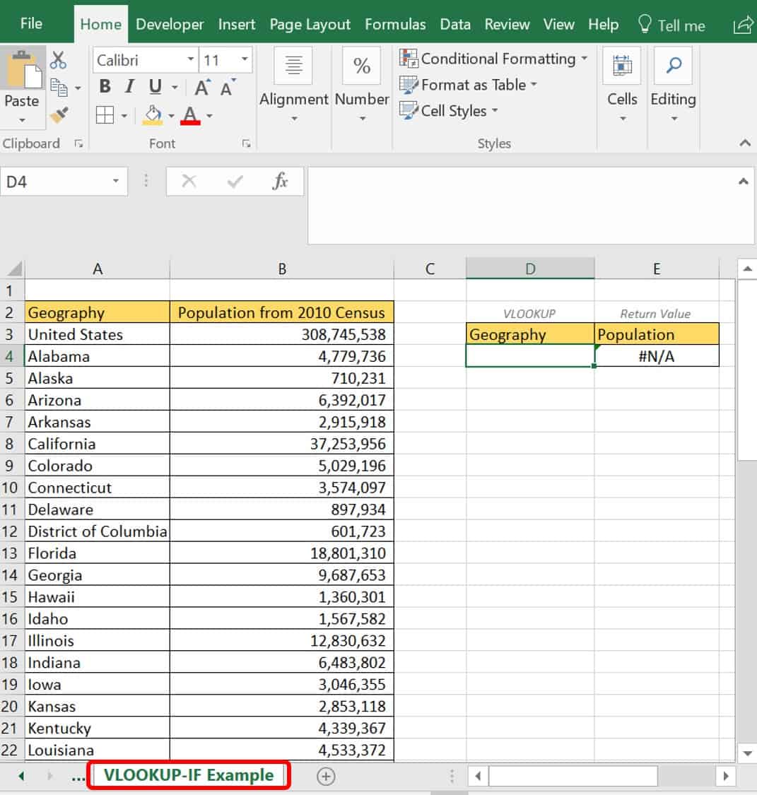
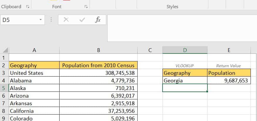
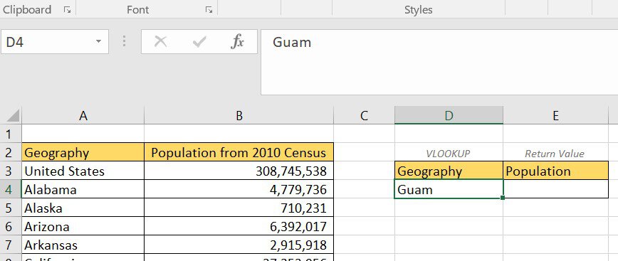
This worksheet shows geography and the population from the 2010 United States Census. Without any value specified in the Geography VLOOKUP box, the return value in the Population box displays the #N/A error. If you type Guam in cell D4, you would also receive this error.

The current formula for this VLOOKUP is =VLOOKUP(D4,A2:B55,2,FALSE), which works well for values found in the data table.
2. To combine the VLOOKUP and the IF function, wrap the VLOOKUP with the IF formula using the ISNA function to check for an #N/A error. The format for an IF function is:
IF(something is true, do something else, do something else because the comparison is false)
IF statements are logic tests that can have two different results based on whether a comparison is true or false. ISNA checks for a #N/A error. The logic for this IF statement is:
IF(there is an #N/A error, enter blank cell, otherwise enter the VLOOKUP result)
Your VLOOKUP statement is used twice in this formula. Type the following arguments in cell D4:
=IF(ISNA(VLOOKUP(D4,A2:B55,2,FALSE)),"",VLOOKUP(D4,A2:B55,2,FALSE))
Here is the IF formula broken down into its three arguments:
Argument | Value | Meaning |
|---|---|---|
Logical_test |
| If the VLOOKUP returns an #N/A error |
Value if true | “ ” | Blank cell |
Value if false |
| Use the VLOOKUP result |
3. Click Enter on the keyboard.
Note: When entering a Geographic area that is not in the data table, the Population cell still returns a blank cell.
VLOOKUP Function Example: How to Combine IFERROR and VLOOKUP
In Excel 2007, Microsoft added the IFERROR function. Compared to the above IF-ISNA function, the IFERROR function requires less time and computing power. In the IF-ISNA function above, you ran the VLOOKUP once to see if it failed, and if it did not fail, you ran it again. The IFERROR function does the lookup only once and allows you to specify what it does if it fails.
The syntax of the IFERROR function is as follows:
=IFERROR(value,value_if_error)
So if Excel checks the value and returns an error, you can choose what value to display. Excel checks for the following errors: #N/A, #VALUE!, #REF!, #DIV/0!, #NUM!, #NAME?, and #NULL!.
Follow these steps to combine the IFERROR and VLOOKUP functions.
1. Click the VLOOKUP-IFERROR Example worksheet tab in the Excel Sample Data file.
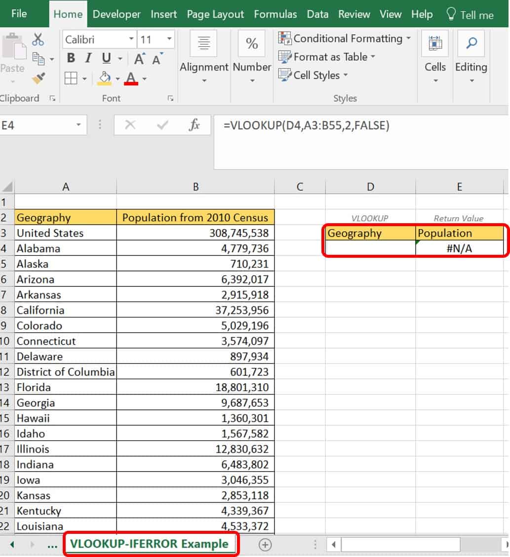
This worksheet shows the data from the 2010 Census by geography with no value specified in the Geography box. But the Population box shows an #N/A error.
2. In cell E4, wrap the current VLOOKUP formula with the IFERROR formula. The VLOOKUP formula is currently =VLOOKUP(D4,A3:B55,2,FALSE). To wrap this with an IFERROR function, type the following arguments around the VLOOKUP:
=IFERROR(VLOOKUP(D4,A3:B55,2,FALSE),"Not Found")
Here are the two arguments in the IFERROR formula:
Argument | Value | Meaning |
|---|---|---|
Value |
| The value the VLOOKUP returns |
Value_if_error | “Not Found” | The value returned if the first argument returns an error |
3. Click Enter on the keyboard.
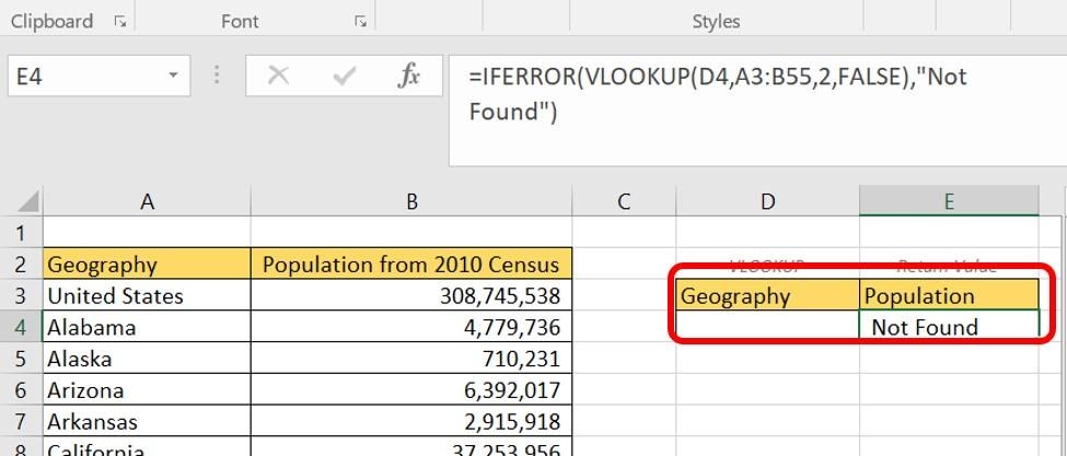
In this example, you have specified that the return value in case of an error is Not Found. The same return would apply if you entered another geography not listed in the table, such as Brazil.
How to Perform a Nested VLOOKUP with Multiple Criteria
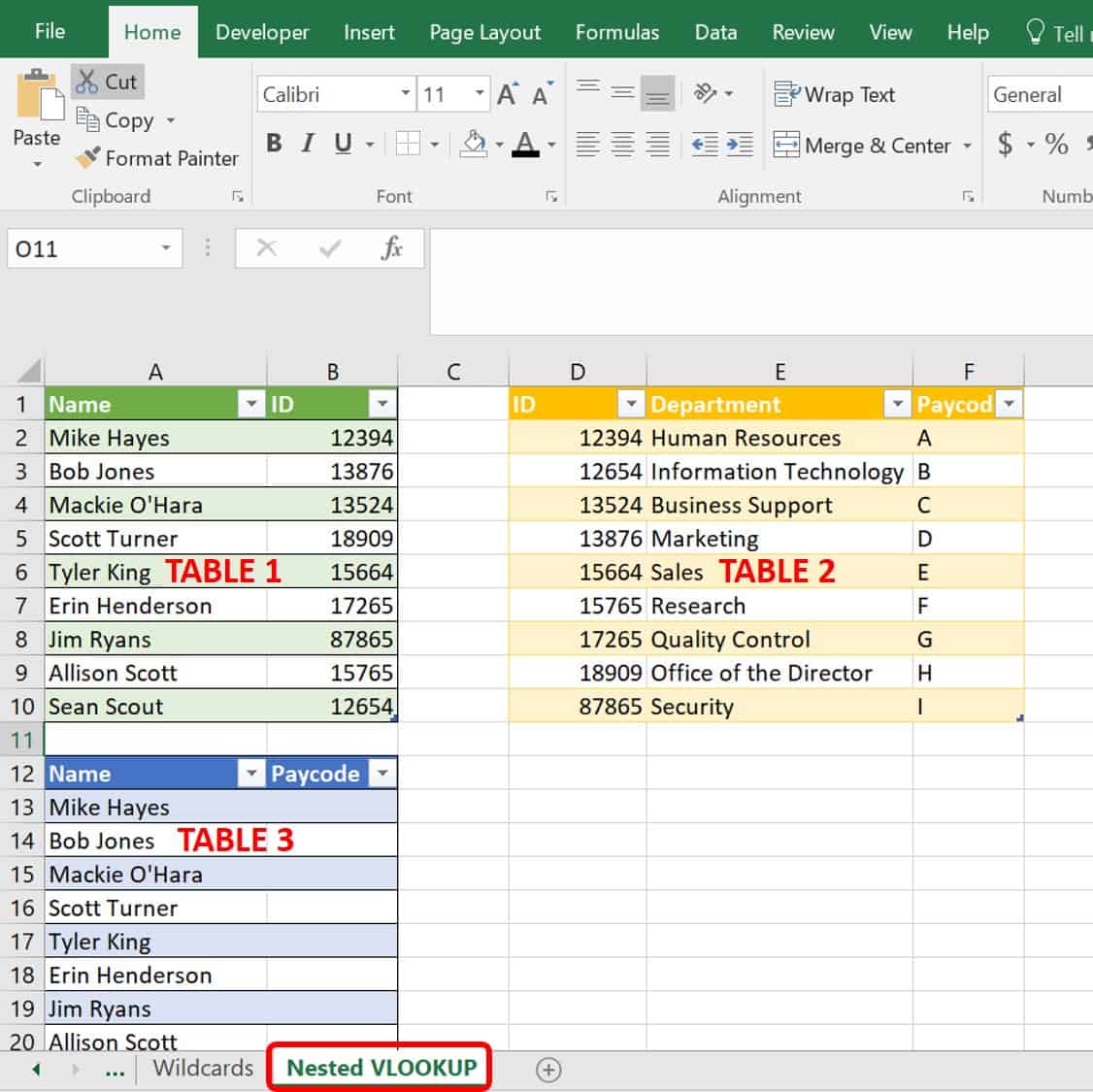
One of the prime requirements of the VLOOKUP function is that your main data table and your lookup table have data in common. However, a table occasionally translates and acts as an intermediary for this data. See the following three tables:
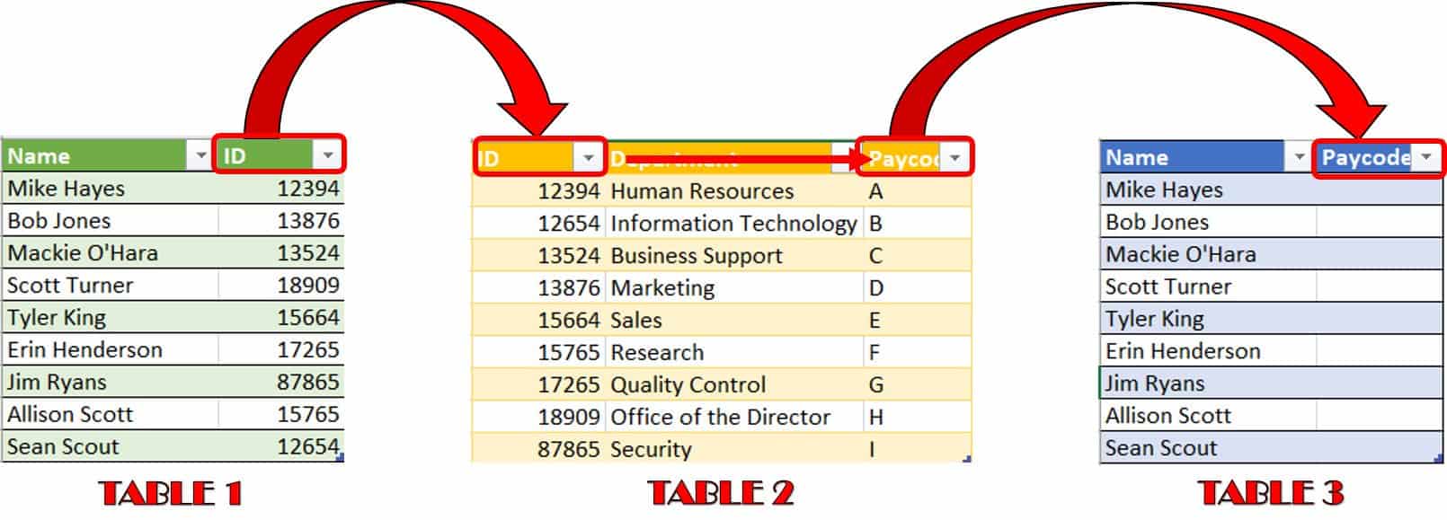
Table 1 has the same column of data available in Table 2, so Table 2 can fill in the data for Table 3 as an intermediary. This is the purpose of nesting formulas: They can draw data from each other.
You must use VLOOKUP in an intermediary step to fill in the data you seek for your final table. Without Table 2, you cannot answer your query. Practically, you are using Table 2 to look up the matching ID to the Paycode and match the Paycode to the Name from Table 1. You will enter the VLOOKUP formula in the Paycode column of Table 3.
Follow these steps to perform a nested VLOOKUP with multiple criteria.
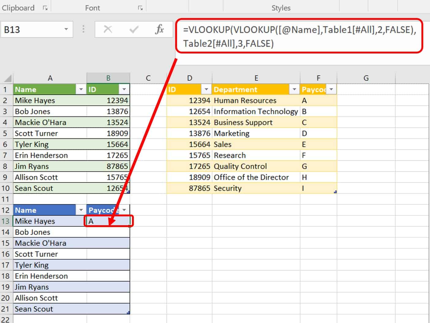
1. Click on the Nested VLOOKUP worksheet tab in the Excel Sample Data file.
2. Type your first VLOOKUP formula in cell B13:
=VLOOKUP(VLOOKUP([@Name],Table1[#All],2,FALSE),Table2[#All],3,FALSE)
The Tables in this Excel worksheet have been named and saved as Tables 1, 2, and 3. The practice of naming the tables changes the cell name in your formulas to the table titles. For example, cell A13 is [@Name] in the formula above. When you specify the whole of a table in Excel formulas, Excel writes it as Table1[#All]. Breaking down this formula, Excel performs the first VLOOKUP first. Nested formulas (those in parentheses) are calculated first. The first formula is:
=VLOOKUP([@Name],Table1[#All],2,FALSE
Argument | Value | Meaning |
|---|---|---|
Lookup_Value | [@Name] | The vertical lookup reference, cell B13 |
Table_array | Table1[#All] | The range of cells Excel looks through to find the lookup reference in the table, Table 1 cells A1:B10 |
Col_index_num | 2 | The column number with the required data |
[range_lookup] | FALSE | The exact value defined |
Without the additional VLOOKUP formula surrounding this VLOOKUP function, your return value would show 12394. However, you wrapped the internal VLOOKUP with another VLOOKUP formula (=VLOOKUP(Return value from first VLOOKUP function),Table2,3,FALSE). Therefore, your return value in cell B13 is A.
3. Copy cell B13 and use Paste Formula to insert it into the reminder of the cells in the Paycode column for Table 3. Click Enter on the keyboard.
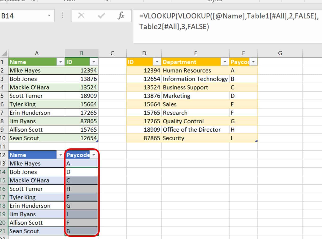
Notice that the formula recognizes that the data is part of a defined table in Excel and does not change based on its cell. This shows the flexibility of Excel tables.
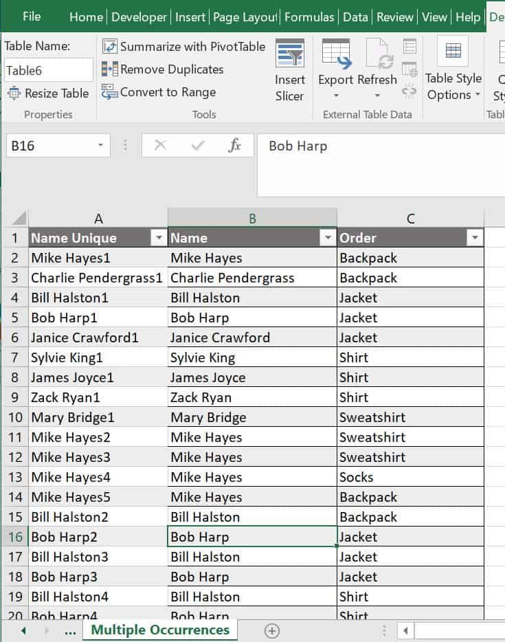
How to Use VLOOKUP to Get Second, Third, or Fourth Occurrences of the Lookup Value
You have already learned that Excel can return only the first matching value in a VLOOKUP. However, some Excel experts want to return other or all occurrences of the matching values. That is, they want to find each unique occurrence, though the data appears to be duplicate. For example, a database has the last several years of orders from a clothing company. Some of the orders are repeats, although they were done at different times and may have been for different items.
Use the following method to make each record unique and show these multiple occurrences. VLOOKUP returns only one value at a time to each cell, but you can make it so that each duplicate becomes unique.
Follow these steps to return other occurrences of the matching value.
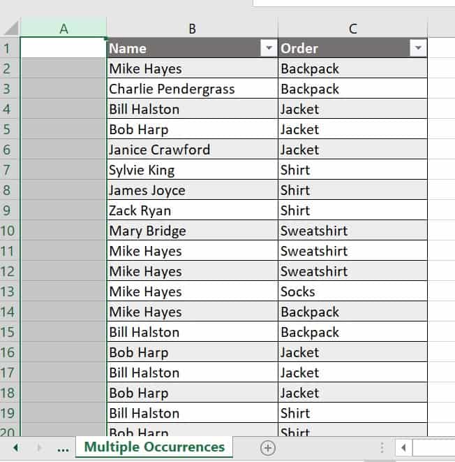
1. Click on the Multiple Occurrences worksheet tab in the Excel Sample Data file.
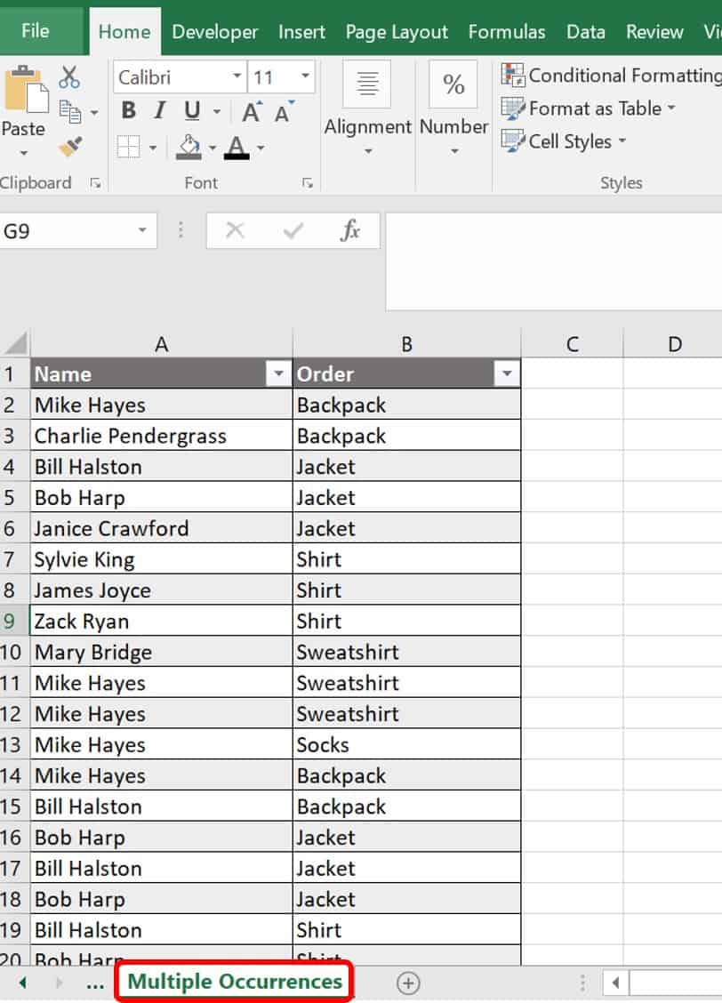
This worksheet displays a sales team and their individual orders to a merchandiser. Column A does not have unique values in every row. The merchandiser wants to know the subsequent purchases for each person.
2. Add a new column to the left of the Name column (Column A) by right-clicking A at the head of the first column and clicking Insert. A new column A is created and the remainder of the table moves to the right.
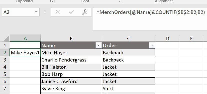
3. Type the following COUNTIF formula in cell A2:
=MerchOrders[@Name]&COUNTIF($B$2:B2,B2)
Here’s the breakdown for the formula:
Value | Argument | Meaning |
|---|---|---|
MerchOrders[@Name] | B2 | Refer to cell B3 |
& | - | Concatenate symbol |
COUNTIF($B$2:B2 | COUNTIF(Range | The range of cells to count unique values |
B2 | Criteria | The criteria that controls which cells are counted |
4. Copy cell A2 and use the Paste Formula option to copy it down the table.
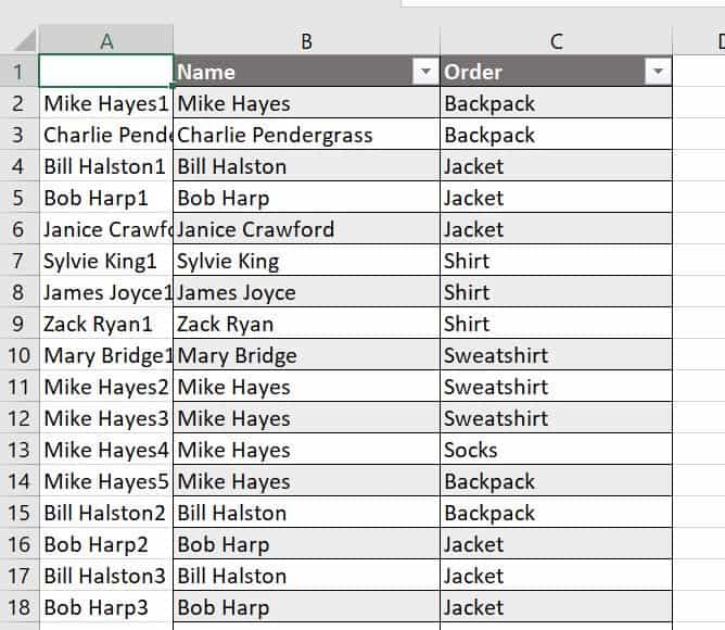
5. Name column A Name-Unique.
6. Click anywhere in the table to reveal the Design tab. Click the Design tab and click Resize Table. This action opens the Resize Table pop-up box. Now, you can add the first column into your predefined table by changing the first letter from B to A as shown below.
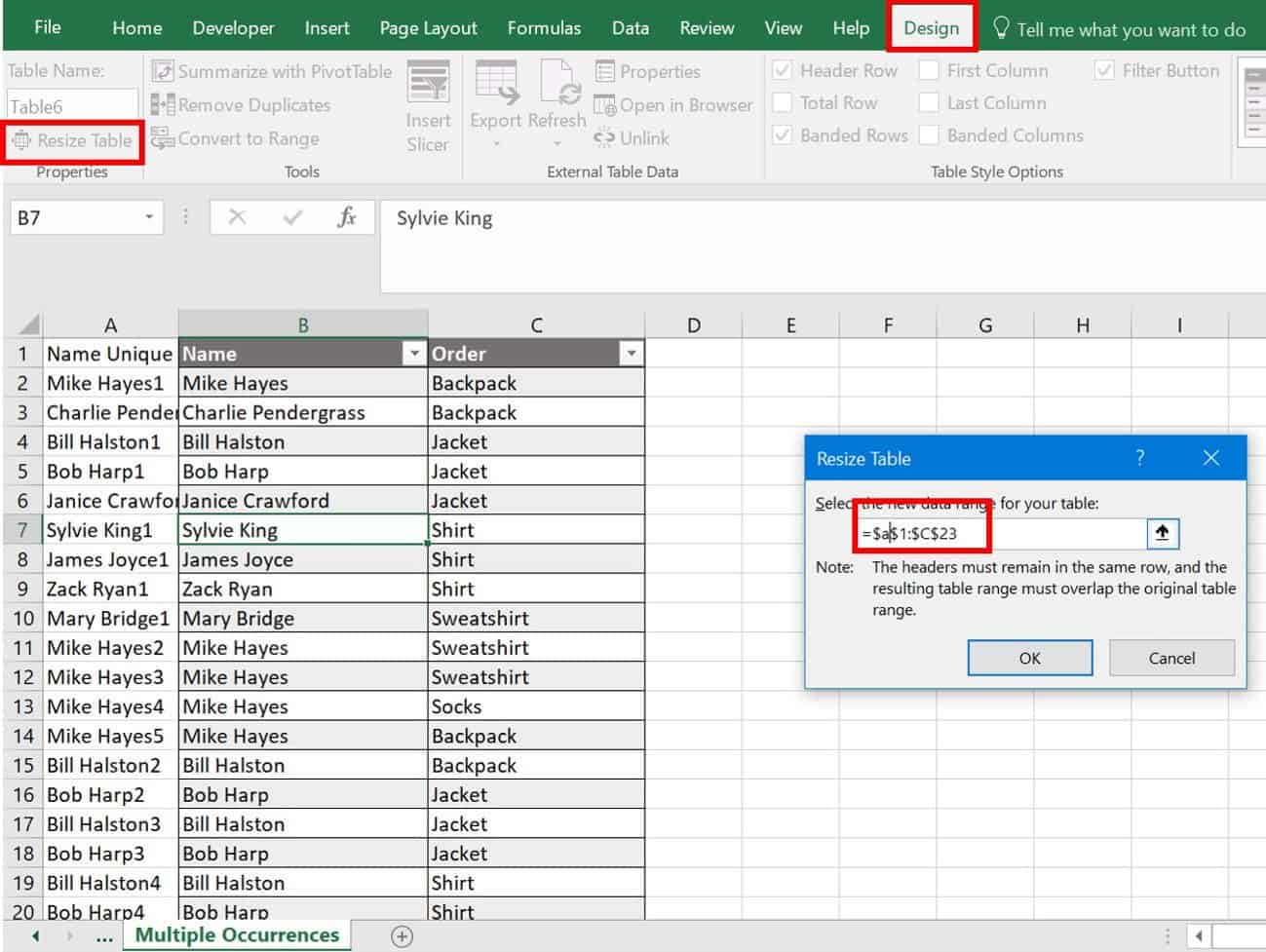
7. Click OK.
8. Use the regular VLOOKUP formula to find your orders. In cell F4, type:
=VLOOKUP(F3,Table6[#All],3,FALSE)
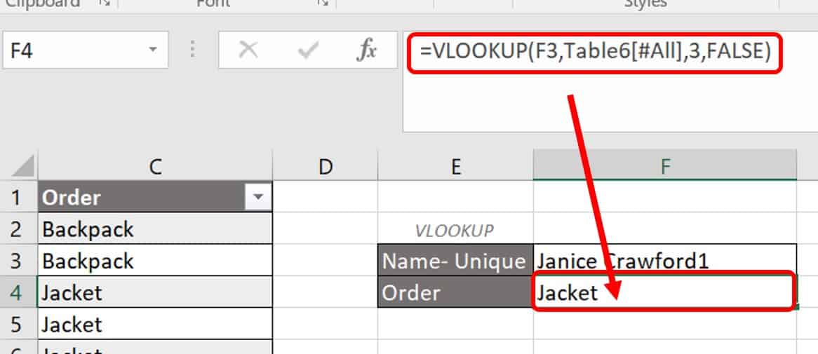
Note: The VLOOKUP formula would not be helpful for retrieving all the matching values for this at once.
How to Combine VLOOKUP and INDIRECT Functions
Using the INDIRECT function with the VLOOKUP returns a range. Use this shortcut if you do not want to constantly change the range of cells when updating your worksheets. In this combined function, you are pulling data from multiple worksheets that have the same formatting. For example, you could use this to combine reports. Normally, you can reference only one additional worksheet in VLOOKUP, but adding the INDIRECT function allows you to reference more worksheets, as long as they have an identical setup.
Follow these steps to combine the VLOOKUP and INDIRECT functions.
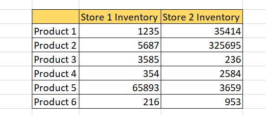
1. Click on the INDIRECT-Summary worksheet tab in the Excel Data Sample file. You also have two additional worksheets for this exercise: Store 1 Inventory and Store 2 Inventory. The naming of the worksheets is crucial, as you need to replicate those names exactly on the Summary worksheet.
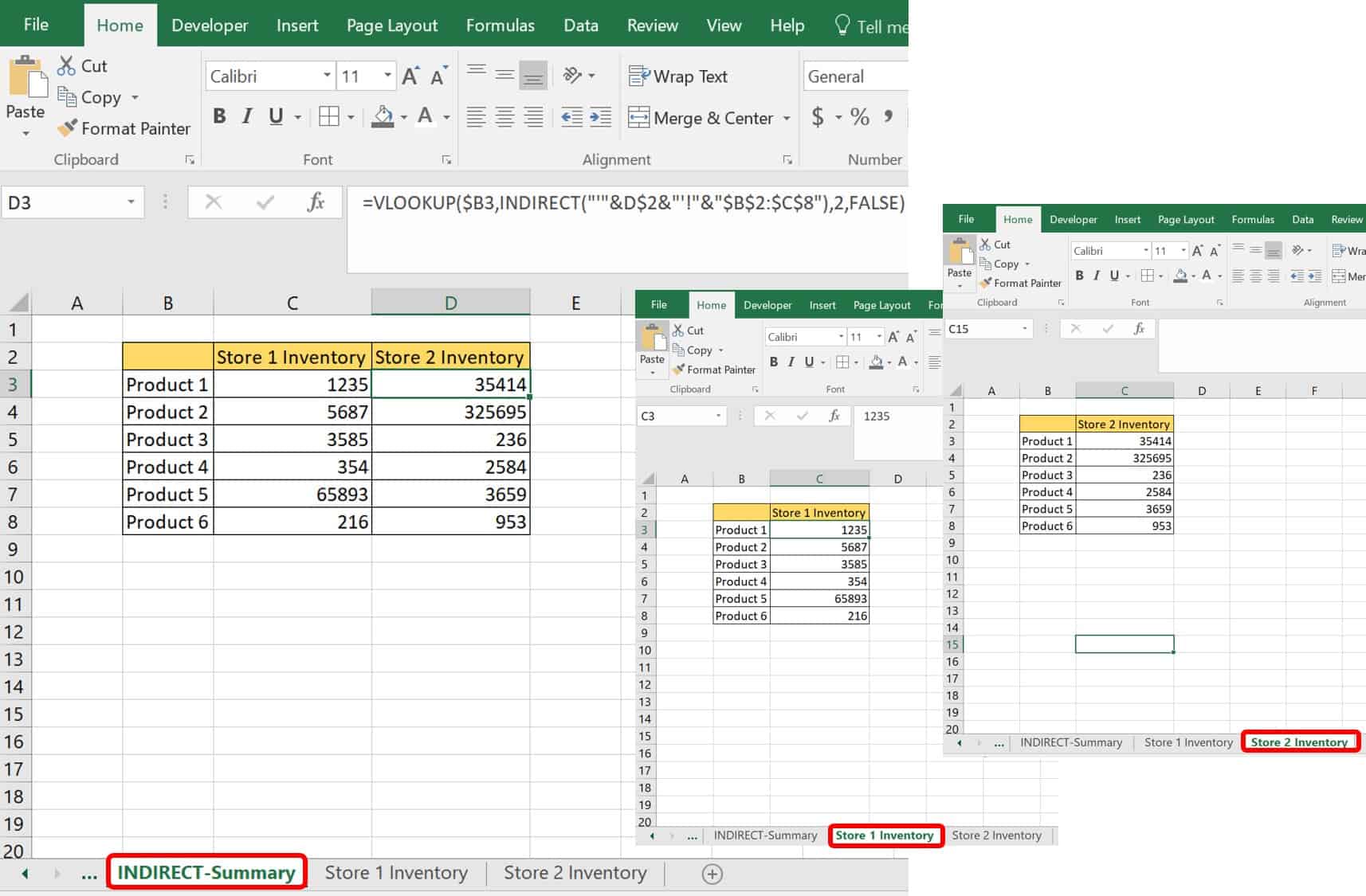
2. On the INDIRECT-Summary worksheet, notice that the two column headers located in cells C2 and D2 match the names of the two worksheets you are pulling data from. You are looking to pull the different stores’ inventory numbers into one tracking sheet: INDIRECT-SUMMARY.
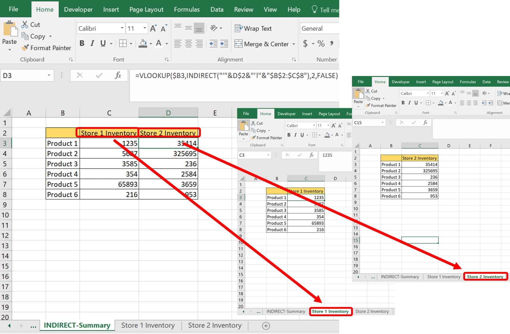
3. In cell C3 of the INDIRECT-Summary worksheet, type the following formula:=VLOOKUP($B3,INDIRECT("'"&C$2&"'!"&"$B$2:$C$8"),2,FALSE)
The VLOOKUP formula is the same as the one you have been writing up to this point. The first argument (Lookup_value) is Product 1 with absolute references $ on the column letter, but not on the row number so that the formula can tile down but not across to the right.
The INDIRECT function is located in the second argument (table_array). INDIRECT functions have two components: the reference text (ref_text) and A1 [a1]. The A1 component is optional and defaults to TRUE when omitted, meaning the text referenced is an A1-style reference. The reference text in this formula is:("'"&C$2&"'!"&"$B$2:$C$8")
This creates a range reference to the cells where we want to pull the data. Here is a breakdown of their functions:
- “ ‘ “: A single quote within double quotes (with spaces added for clarity) precedes the sheet name in case there are space characters in the worksheet name.
- &: Concatenate.
- C$2: The absolute reference to cell C2, which is the name of the worksheet we are referencing.
- “!”: The exclamation point surrounded by double quotes means we are looking for another worksheet.
- &: Concatenate.
- "$B$2:$C$8": The data table’s address for the data return we are seeking.
4. Click Enter on the keyboard.
5. Copy cell C3 and use the Paste Formula function in the remainder of the Summary table.
Using INDEX-MATCH Instead of VLOOKUP Sample
Many users like and are comfortable with VLOOKUP because they learned it early in their Excel education. It also performs the function they need. INDEX-MATCH is another lookup function when you nest functions. Here are three reasons why VLOOKUP is not the best choice for this use, and INDEX-MATCH is a better option for a lookup function:
- You need a formula that can look right to left.
- You have an enormous number of columns.
- Your spreadsheet computation is too slow.
The MATCH function searches for a specific item in a cell range and returns the position of that item. The syntax is MATCH(lookup_value,lookup_array,[match type]). Use this function alone if you need the position of an item, but not the actual item.
The INDEX function provides the value within a table, range, or array. The syntax for an INDEX function is INDEX(array,row_num,[column_num]). You can use this syntax in a two-dimensional lookup, as it gives you the opportunity to specify both the row and column location. In a nutshell, INDEX provides the value located at an exact position.
Follow these steps to use INDEX-MATCH for a lookup.
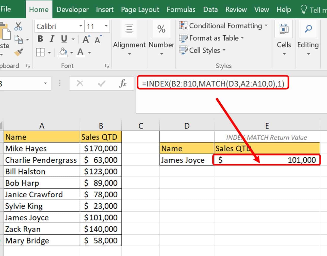
1. Click on the INDEX-MATCH worksheet tab in the Excel Data Sample file.
As you can see, there is a list of the sales team’s quarterly sales to date (Sales QTD).
2. To perform a lookup with INDEX-MATCH, type the following formula in cell E3:
=INDEX(B2:B10,MATCH(D3,A2:A10,0),1)
Breaking down this formula, you have the MATCH nested in the INDEX formula. Excel performs this function first:
=MATCH(D3,A2:A10,0)
Argument | Value | Meaning |
|---|---|---|
Lookup_value | D3 | Where the reference value to lookup is located |
Lookup_array | A2:A10 | The data table where the lookup value may be found |
[Match type] | 0 | This means you want an exact match |
For the INDEX function:
=INDEX(B2:B10,MATCH,1)
Argument | Value | Meaning |
|---|---|---|
Array | B2:B10 | Where the reference value to lookup is located |
Row_num | MATCH | The value returned by the MATCH function – which is the row number of the reference data |
[Column_num] | 1 | The column number of the reference data |
3. Click Enter on the keyboard.
VLOOKUP Examples in Google Sheets
Google Sheets is an Excel competitor, but allows more collaboration options as it was born in the cloud. Many functions in Excel are also in Google Sheets, and many Excel spreadsheets may be converted to Google Sheets and vice versa. However, you cannot use one program as a reference for the other. For example, in the case of VLOOKUP, you may not add an Excel spreadsheet reference into the formula on your Google Sheet and expect it to pull data from that Excel sheet.
Certain functions in Google Sheets work in the same way they do in Excel. VLOOKUP is one of those functions.
How to Perform a VLOOKUP from a Different Google Sheet
Follow these steps to perform a VLOOKUP from a different Google Sheet.
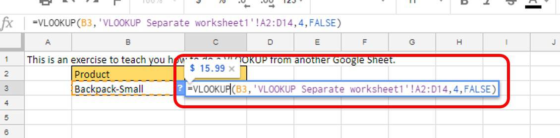
1. Click on VLOOKUP Separate worksheet1 worksheet tab in the Google Sheet Sample file. (Note: Some formulas shown in this tutorial already appear in the Google Sheet Sample file.) For this exercise, you also have a VLOOKUP Separate worksheet2 to use.
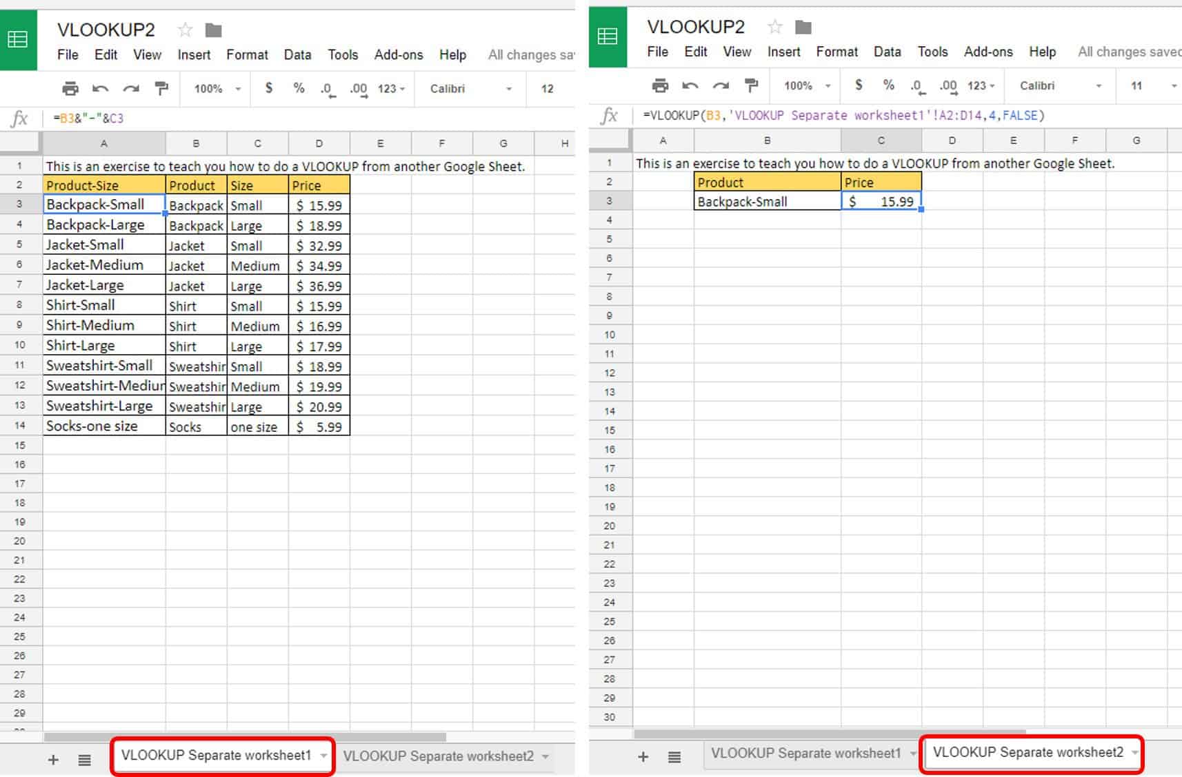
2. Type the following formula into cell C3 on VLOOKUP Separate worksheet2:
=VLOOKUP(B3,'VLOOKUP Separate worksheet1'!A2:D14,4,FALSE)
Let’s break down this formula:
Argument | Value | Meaning |
|---|---|---|
Search_key | B3 | Where to look up the search value |
Range | 'VLOOKUP Separate worksheet1'!A2:D14 | The location of the table data for Google Sheets to sort through |
Index | 4 | The column number to find the data |
Is_sorted | FALSE | The exact match that is not sorted |
To signify that you are looking at data from another sheet, the sheet name for the Range is surrounded by single quotes (‘) and followed by an exclamation point (!).
Google Sheets does a few things differently than Excel:
- The formula in the overhead bar is colored to match the formula in the cell and remains that color.
- Google Sheets provides a return value as you type the formula in a call-out box above the formula.
- Google Sheets automatically saves your work and updates from multiple users in real time, and it supports VLOOKUP with wildcard characters.
- The formulas are defined slightly differently than those in Excel. They work in the same manner, but they are meant to be more intuitive to understand.
How to Perform a VLOOKUP Across Sheets in Smartsheet
Smartsheet is a work management platform that allows you to use higher-level functions across your sheets. Since Smartsheet does not store sheets in the traditional “workbook” format, you can reference any sheet you can access with your login address.
Follow these steps to perform a VLOOKUP across sheets.
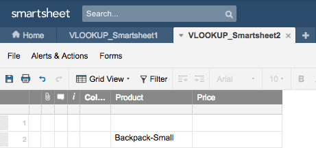
1. Click on the Smartsheet VLOOKUP_Smartsheet1 and view. This sheet has information imported from a product database on products and their correlating prices. For this exercise, see also VLOOKUP_Smartsheet2, which has designated space for a VLOOKUP for this example. In this sample, you want to look up data from VLOOKUP_Smartsheet1 and add it to VLOOKUP_Smartsheet2 using the VLOOKUP formula.
2. With Smartsheet, you can either type in the whole formula or use the function button that Smartsheet located in the Numbers section on the sheet. In this example, you will use the Function button. Open the VLOOKUP_Smartsheet2 sheet and click on the Price2 cell, then click on the drop-down arrow next to the Function button. Click Advanced Functions and VLOOKUP. You can also find the VLOOKUP function under Functions/All Functions.
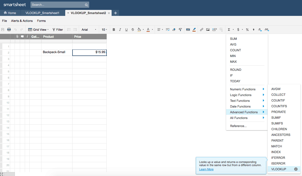
The VLOOKUP formula loads into the Price2 cell, with notes on syntax and examples.
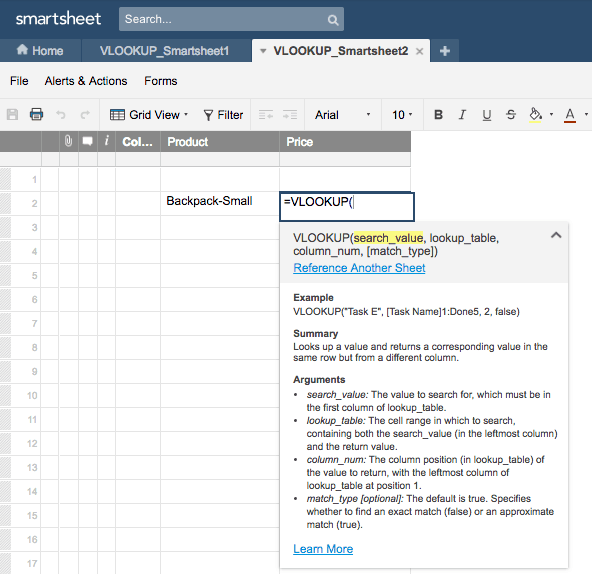
The syntax for VLOOKUP in Smartsheet is as follows:
=VLOOKUP(search_value,lookup_table,column_num,[match_type]
The VLOOKUP method in Smartsheet is similar to that of Excel and Google Sheets, but is more intuitive and user-friendly. The currently required argument in the formula is highlighted. As with Excel, you can select the cells where your current argument is located or type the argument directly into the formula. Separate each argument by typing a comma (,).
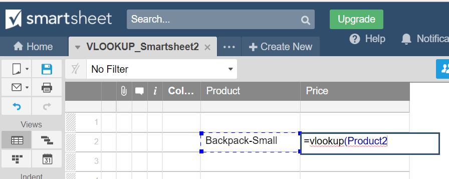
3. The formula for this function is the following:
=VLOOKUP(Product2,{PriceTable},4,false)
Argument | Value | Meaning |
|---|---|---|
search_value | Product2 | The value you are looking to match |
lookup_table | {PriceTable} | The data table that your information is drawn from |
column_num | 4 | The column number in the data table that you reference for the return value |
[match_type] | false | This is an exact match and must include a space after the comma |
Select cell Product2 for the first argument and follow the selection with a comma (,).
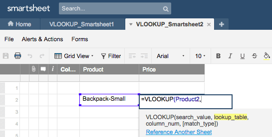
4. Once you type the comma after the first argument, the second argument is highlighted in the help pop-up box. To access a data table that is present on another sheet, you must click the Reference Another Sheet hyperlink.
The Reference Another Sheet pop-up box appears. Choose from all the sheets that your Smartsheet email allows you to access. You can choose data from any of these sheets. For this example, choose VLOOKUP_Smartsheet1.
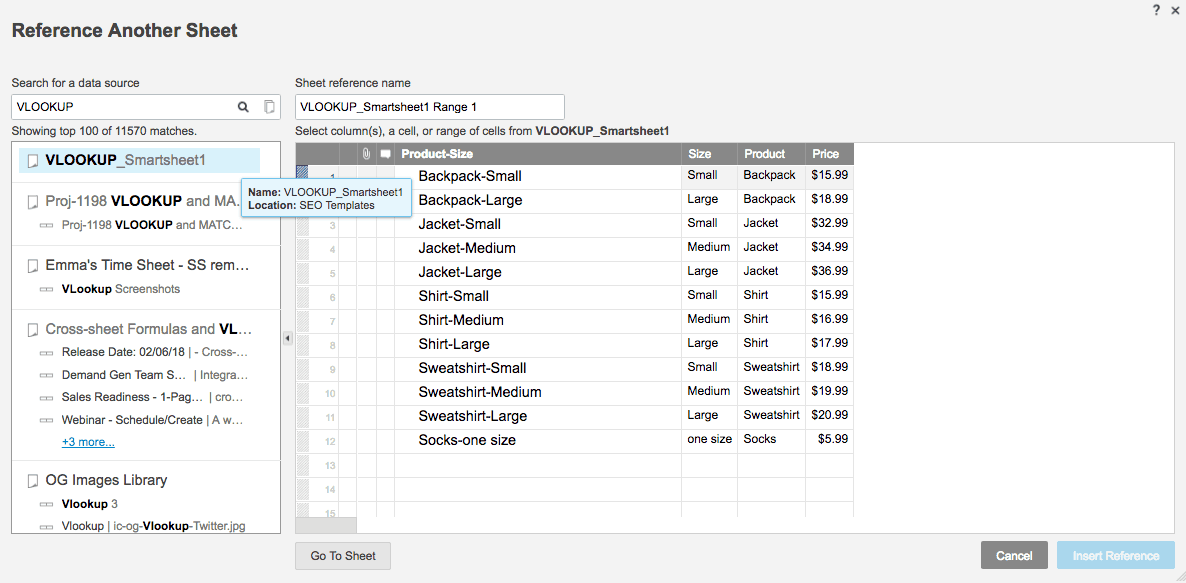
5. Click VLOOKUP_Smartsheet1. To select your table range, Smartsheet recommends clicking the column header of the columns you want to include. To select multiple columns, hold down the Shift or Ctrl key on the keyboard and click it with your mouse. Click and highlight all the cells. Once the cell range is highlighted, you can also change the name of the range in the Sheet Reference Name box to make it easier to read in your formula. For this exercise, replace VLOOKUP_Smartsheet1 Range 6 with PriceTable. When you name your range, remember that Smartsheet does not allow you to submit a name of a cell or table that is already in use in that sheet.
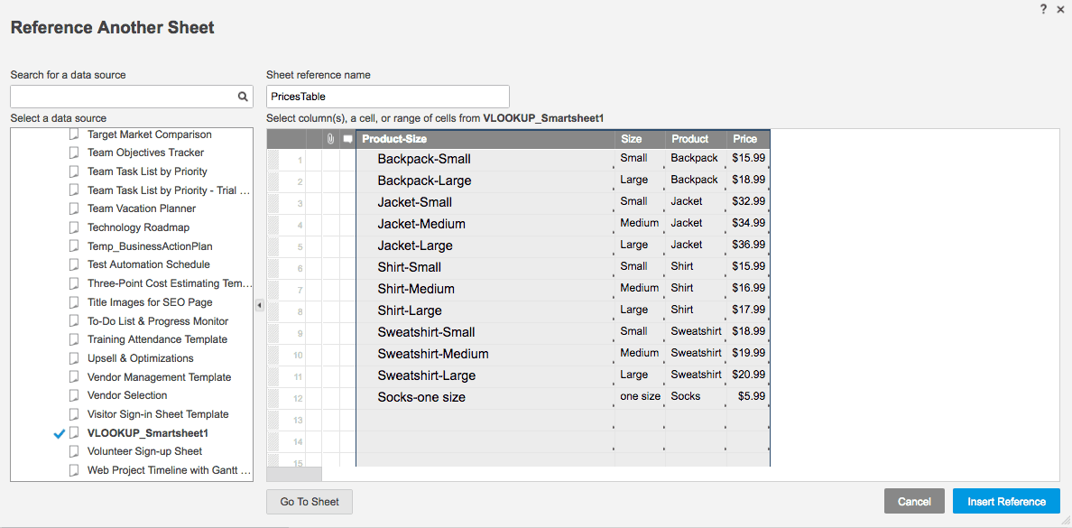
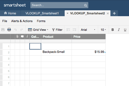
6. Click Insert Reference on the Reference Another Sheet pop-up box. This action closes the pop-up and returns you to VLOOKUP_Smartsheet2.
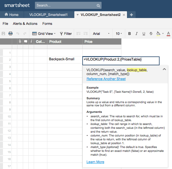
Since you are referencing a data table that comes from another sheet, the lookup_table reference is surrounded by curly brackets {}.
7. You can type the last two arguments in this function manually. Close your second argument with a comma (,) and type 4, then false. The last argument must be lowercase.
8. Type the close parenthesis ) and click Enter on the keyboard to complete this function.
For more information about VLOOKUP function across sheets, watch this video.
In Smartsheet, the following are best practices and tips for using formulas across sheets:
- Use cross-sheet formulas on any sheet you can access. Note: You must have at least editor access on the destination sheet and viewer access on the source sheet.
- Reference the entire column in your formula for accuracy. This way, if your data table changes, Smartsheet can recognize the parameters in your formulas, and the formulas will stay intact.
- Custom-name ranges in cross-sheet formulas: This practice allows you and colleagues viewing your formulas to better identify the ranges selected.
- Know your limits. A maximum of 25,000 cells is available for cross-sheet references in these formulas in Smartsheet. This is significantly larger than past cell links maximums, which were 5,000.
- Use cell links when calculations are not necessary. Cell links enable users to input data from a cell in one sheet into another sheet, without the benefit of a calculation. If you need to use calculations with your data to perform any number of higher-level functions, go with functions such as VLOOKUP, SUMIF, or COUNTIF.
Connect Data Across Your Work with VLOOKUP in Smartsheet
Empower your people to go above and beyond with a flexible platform designed to match the needs of your team — and adapt as those needs change.
The Smartsheet platform makes it easy to plan, capture, manage, and report on work from anywhere, helping your team be more effective and get more done. Report on key metrics and get real-time visibility into work as it happens with roll-up reports, dashboards, and automated workflows built to keep your team connected and informed.
When teams have clarity into the work getting done, there’s no telling how much more they can accomplish in the same amount of time. Try Smartsheet for free, today.
