Basic to Advanced VLOOKUP Uses and Formulas
VLOOKUP is a powerful Excel formula that you can use to capture data from a complex database and deliver it where you need it. When used correctly, it can save you a ton of time and make you a more efficient and proficient Excel user. The VLOOKUP syntax is:
=VLOOKUP(lookup_value,table_array,col_index_num,[range_lookup])
Argument | Meaning |
|---|---|
Lookup_Value | The reference value, which can be a text, a numerical string, or a cell whose value you want to reference. |
Table_array | The overall data table. As such, the reference value you are looking up should be in the first column of this table, column 1, so Excel can move to its right and search for the return value. |
Col_index_num | The column number where the return value is located. This value starts at 1 and goes up relative to the number of columns in your table. |
[Range_lookup] | The fourth value is in brackets because it is not a mandatory argument to make this function work. Brackets in Excel syntax mean that the argument is optional. If you don’t complete this value, Excel autoselects TRUE (or 1), which means that you are not looking for an exact match to your reference value, but an approximation. Using TRUE as the value is not recommended for text returns. |
To use VLOOKUP, you’ll need to supply (at a minimum) the first three pieces of information. To input formulas in Excel, you can type them directly into the cells or use the function wizard. It is difficult, however, to write formulas in the wizard and check them as you go (pressing F9). One tip with Excel is to write from the inside out. Since Excel computes the innermost function(s) first, you should understand what each returns before you wrap it into another function.
Another tip when preparing your data to write formulas is to name your table ranges. For example, cells A1:B18 refer to the following table:
In a formula, refer to the above section of data as A1:B18 and add absolute value signs ($) to maintain this table ($A$1:$B$18) as it is seen here when you drag formulas around a worksheet. An even better way to maintain the reference for this table is to transform it into an Excel table by selecting Creating a Table on the Insert tab and renaming it in a manner consistent with its purpose. For more information on creating tables in Excel, see this article.
In this guide, we’ll instruct you to select and drag formulas. To accomplish this task, click the cell and a green box will appear.
Hover over the cell; you will see a black cross that you will then select and drag through connected cells to automatically paste formulas that are relative to your new cells’ positions. Use absolute values ($) when necessary. You can save time and energy by writing formulas that can be used to populate other cells.
If you’re new to VLOOKUP, we encourage you to read How to Use VLOOKUP: Step-by-Step Tutorials, Tip Sheets, and More and Get Ahead with Excel: An Intermediate Guide with VLOOKUP Examples, Formulas, Syntax, and Practice Samples to get a grasp of its basic functionality.
How to Pull Data from One Excel Sheet to Another
Pulling data from one Excel worksheet to another is a matter of writing the address of the data table into the formula correctly. When performing VLOOKUPs from one worksheet to another in the same workbook, you can enter the data table’s address into the formula using either of these options:
- While writing the formula, select both the worksheet with the data table in it and the data table. Excel automatically writes the correct address of the data table into the formula.
- Write the location of the data table directly into the formula using the following format: ‘Name of Sheet’!(data table). For example, to request Excel look up a data table in cells A1:C10 from the worksheet called VLOOKUP, you would write ‘VLOOKUP’!A1:C10. The single quotes surrounding the name of the worksheet and the exclamation point signal to Excel that it must draw the table from another sheet.
For more information on how to reference data in another workbook, see here.
Can You Perform a VLOOKUP from Another Workbook?
Similar to pulling data from one worksheet to another, you can also pull data from one workbook to another. In this case, make sure that the workbook with the data you are referencing is open when you write your formula. Once your formulas are in place and saved, Excel will reference its location. If you move the workbook and save it in another location, you will need to relink it to your formula. Here’s how to create a VLOOKUP formula that pulls data from another workbook:
- While writing the formula, select the worksheet that has the correct data table and select the data table. Excel automatically writes the correct address of the data table into the formula.
- Write the address of the data table directly into the formula using the following format:
‘[Name of Workbook.xlsx]Name of worksheet’!(data table)
For example, to look up a data table reference in cells A1:C10 on a worksheet called VLOOKUP located in a workbook called VLOOKUP3, the formula is:
‘[VLOOKUP3.xlsx]VLOOKUP’!A1:C10
The brackets surround the workbook name, the single quotes surround the name of the worksheet, and the exclamation point signals to Excel that it must draw the table from another workbook and worksheet.
For more information on referencing data from another workbook, see here.
How to Compare Two Columns in Excel
Follow these steps to compare two columns in Excel.
1. Click the Compare two columns worksheet tab in the VLOOKUP Advanced Sample file .
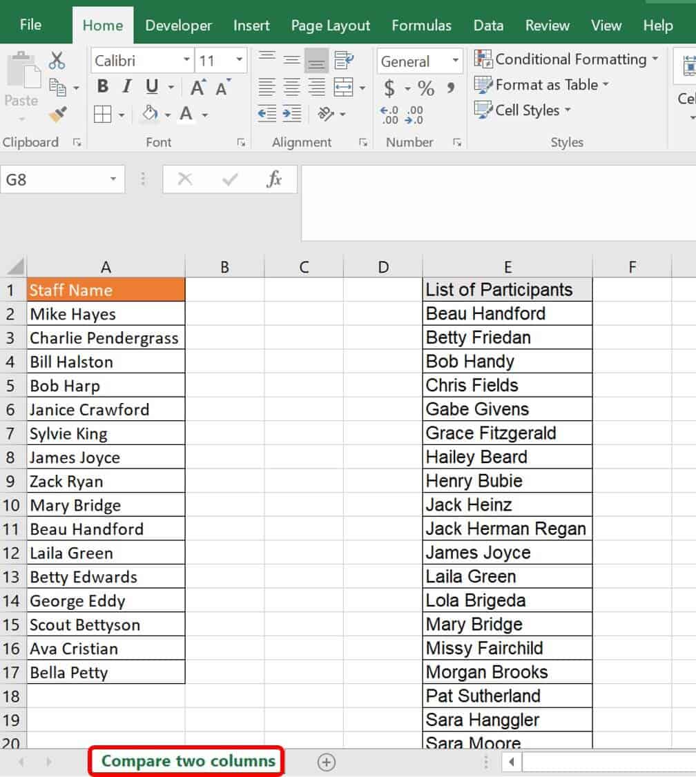
You’ll see a list of staff members in a department. In this example, you want to compare these names to the list of participants from your company’s annual field day to determine who you need to thank for their help. We have a List of Participants column and a separate list of employees in the department on the worksheet. The lists don’t necessarily need to be on the same worksheet, but for visualization purposes, we placed them here. As noted above, you could also perform the search by referring to a list in another worksheet or workbook; just follow the syntax for these functions above.
2. Add columns in your workbook so you have space for results.
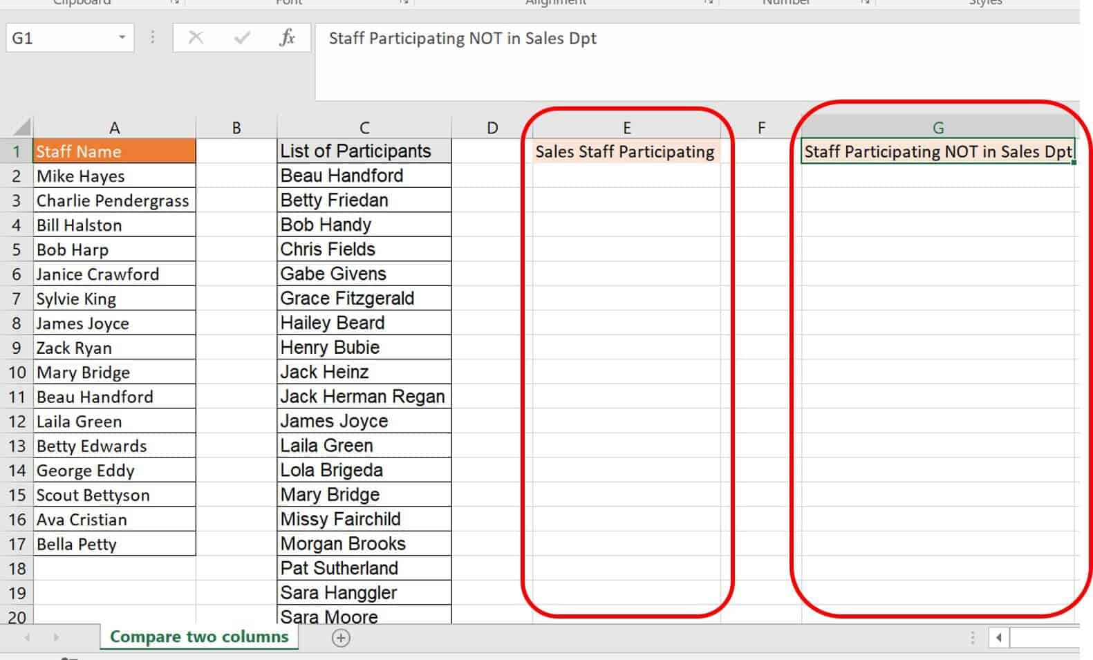
In this example, label the extra columns Sales Staff Participating and Participants NOT in Sales Dpt. The first extra column is for the values duplicated in the two columns, and the second is for identifying the unique values in column C (those who participated, but are not members of the sales department).
3. Type the first VLOOKUP formula in cell E2:
=VLOOKUP(A2,C:C,1,FALSE)
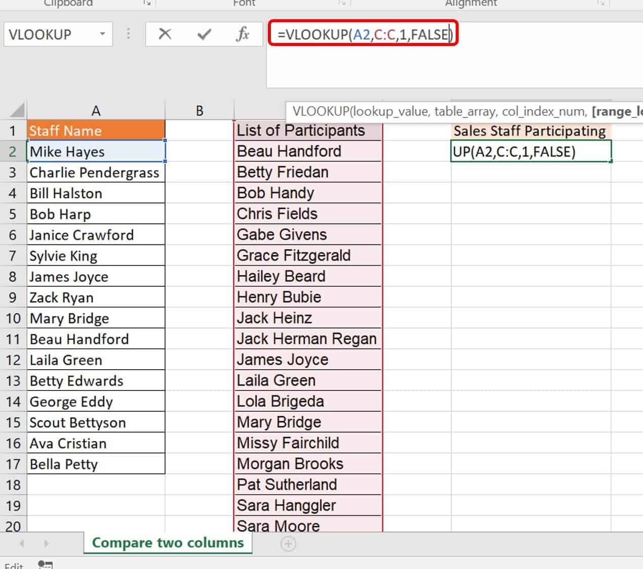
Breaking down this formula:
Argument | Value | Meaning |
Lookup_Value | A2 | The Staff Name of reference you are looking to see in the List of Participants |
Table_array | C:C | C:C refers to column C (List of Participants), which you are checking your reference name against. |
Col_index_num | 1 | This is the column reference number. Since your data table has only one column, the column number is 1. |
[Range_lookup] | FALSE | FALSE means that you are looking for an exact value. |
4. Click Enter on your keyboard and drag the VLOOKUP formula down through cell C17.
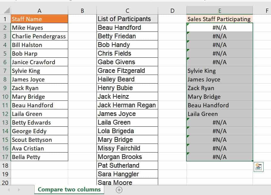
As you can see, the staff that participated in field day showed up by name in column E. The remainder of your sales staff elicited a #N/A error because their names were not listed as participants in column C.
How to Get VLOOKUP to Return a 0 Instead of #N/A
In the above example, you compared two lists to find an overlap. This option provides the data you need, but also gives you #N/A errors where the data does not overlap. As an Excel expert, you know this means that your formula was successful. However, other people looking at this may think #N/A means something is wrong.
For a better-looking list, you can mask the #N/A errors by wrapping your VLOOKUP formula with an IFERROR function.
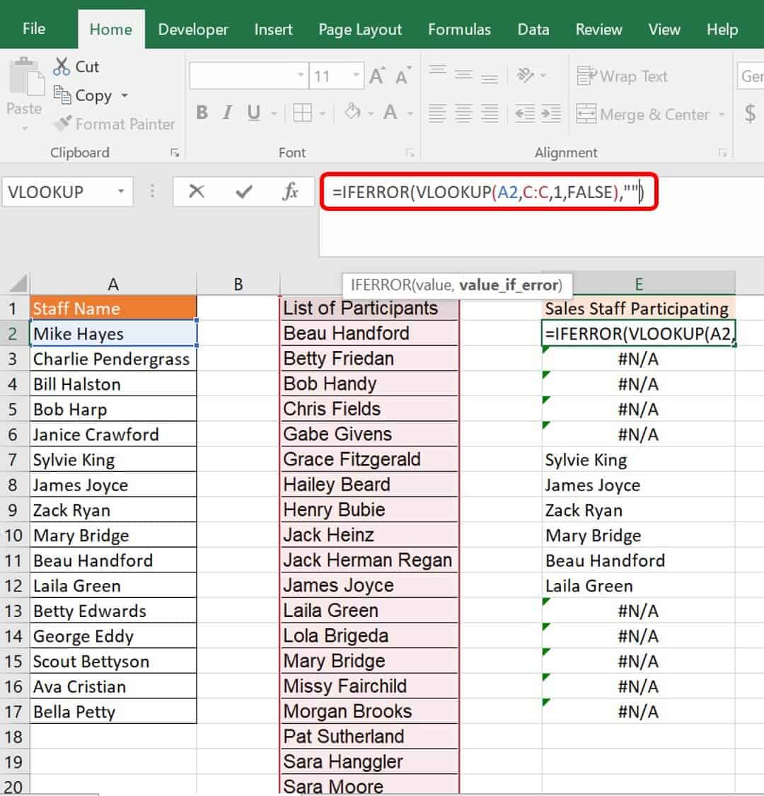
The IFERROR formula wrap tells Excel that if a VLOOKUP formula returns an error to return a blank cell. You could also easily return a zero (0) or another string such as the phrase Not present. The new formula is:
=IFERROR(VLOOKUP(A2,C:C,1,FALSE),””)
1. Click cell E2 and enter the formula =IFERROR(VLOOKUP(A2,C:C,1,FALSE),””) and click Enter on your keyboard.
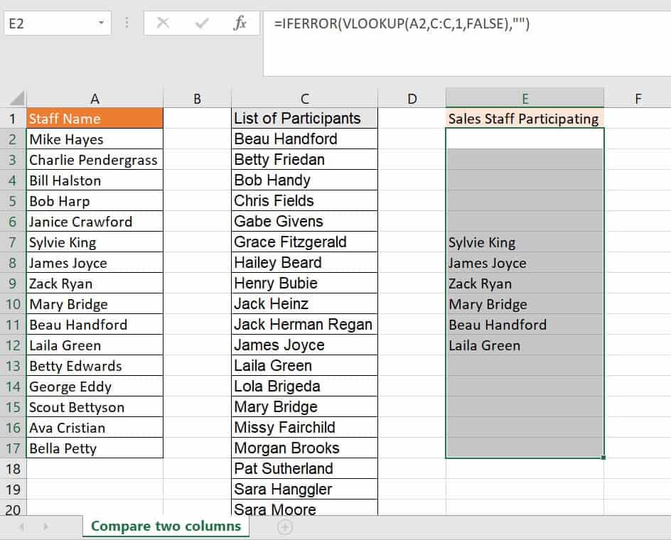
This returns a list of your sales staff who participated without any visible errors.
2. To complete your second inserted column, column G, or the List of Participants NOT in Sales Dpt, type a VLOOKUP formula in cell G2. This formula will be:
=IF(ISERROR(VLOOKUP(C2,A:A,1,FALSE)),C2,"")
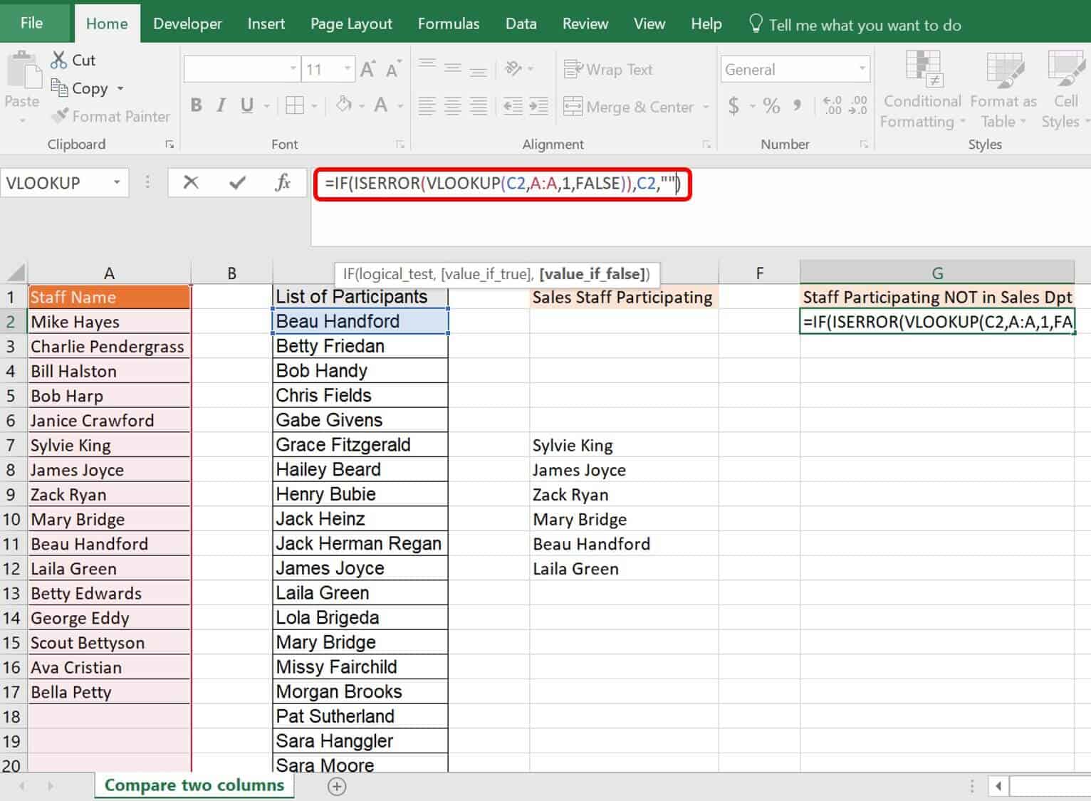
This method is slightly more complex because you wrapped the formula first in an ISERROR function, then in an IF function. Excel performs functions from inside out. For the formula in cell G2, Excel performed the functions in the following order:
Order Excel Performs | Function | Formula | |
1 | VLOOKUP |
| |
2 | ISERROR |
| |
3 | IF |
| |
Each function looks at the return from and bases its formula on the prior function. The VLOOKUP returns either a name from column A or an #N/A error. The ISERROR function looks at this VLOOKUP return and returns TRUE if there is an error (which would be an #N/A error here), and FALSE if there is no error. The IF function takes the ISERROR return and returns what you specify for each value of TRUE or FALSE. In this case, you specified a TRUE value of the value in column C and a FALSE value of a blank (“”) value.
3. After you enter the new formula, click Enter on your keyboard and drag the formula down through cell G23 to cover your whole list of participants.

This provides a list of participants who are not in the sales department.
Overall, the VLOOKUP returns the data that it matches; otherwise it gives you an error message. Adding other functions around VLOOKUP such as IFERROR, ISERROR, ISNA, and IF gives you a way to evaluate the VLOOKUP return and show what’s needed in the cell. You can even include a message or a zero (0) in the quotes. This combination is an effective and quick way to compare data in different columns and present it as you need.
One final type of error is the #NUM! error. Excel produces this error when it expects but does not receive numerical data — for example, entering non-numerical characters such as %, $, or commas (,). This type of symbol is viewed in the formatting of a cell but should not be manually entered. To remove such errors, review the characters and formats of your cells.
How to Create VLOOKUP Using Multiple Criteria and Values
One of the main limiting problems with VLOOKUP is that it only allows you to look for a single value. However, the real world often requires you to use two or more criteria when looking up data from a database.
Follow these steps to create a VLOOKUP using multiple criteria.
1. Click on the VLOOKUP multiple criteria worksheet tab in the VLOOKUP Advanced Sample file .
Download VLOOKUP Advanced Sample file
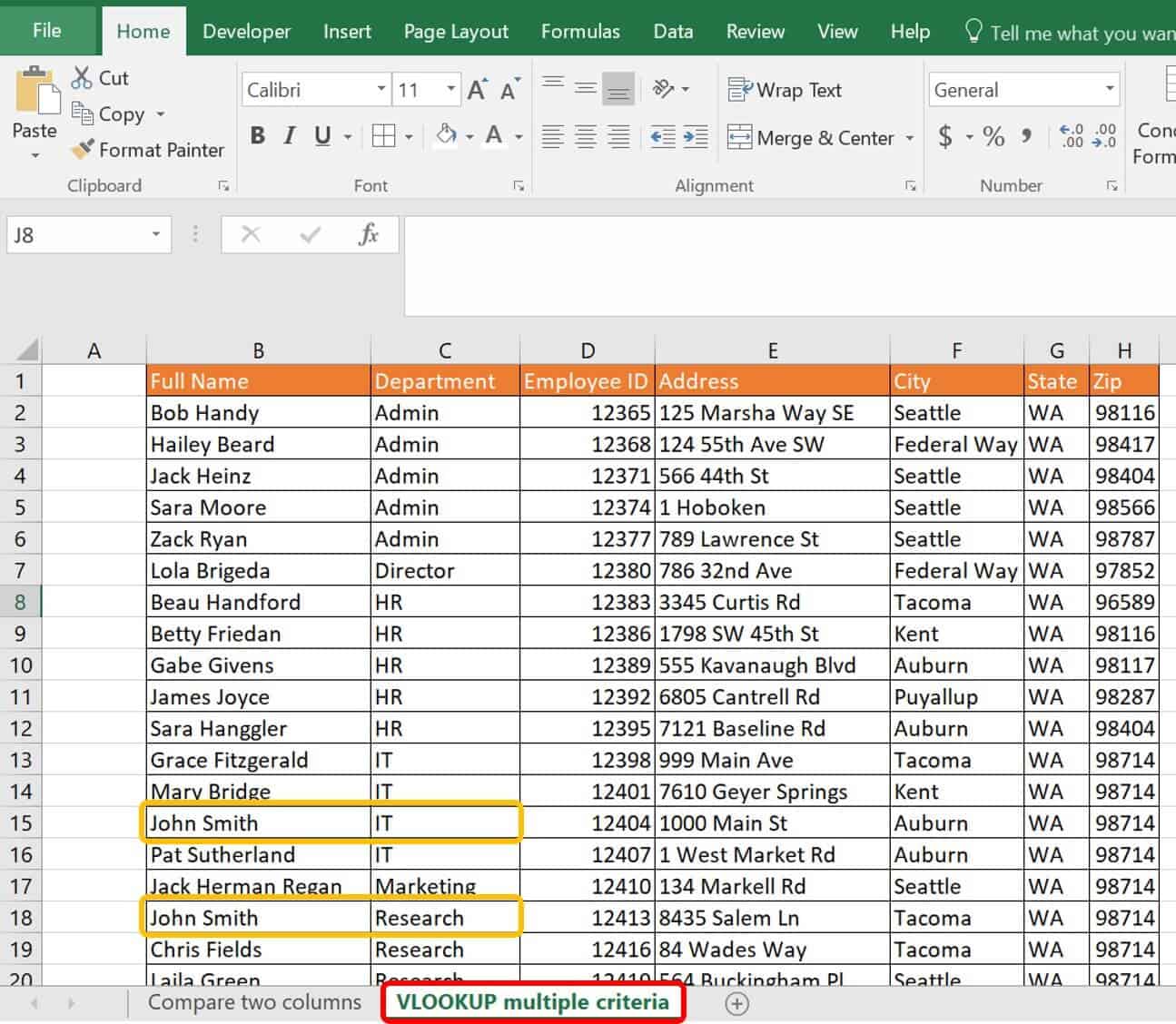
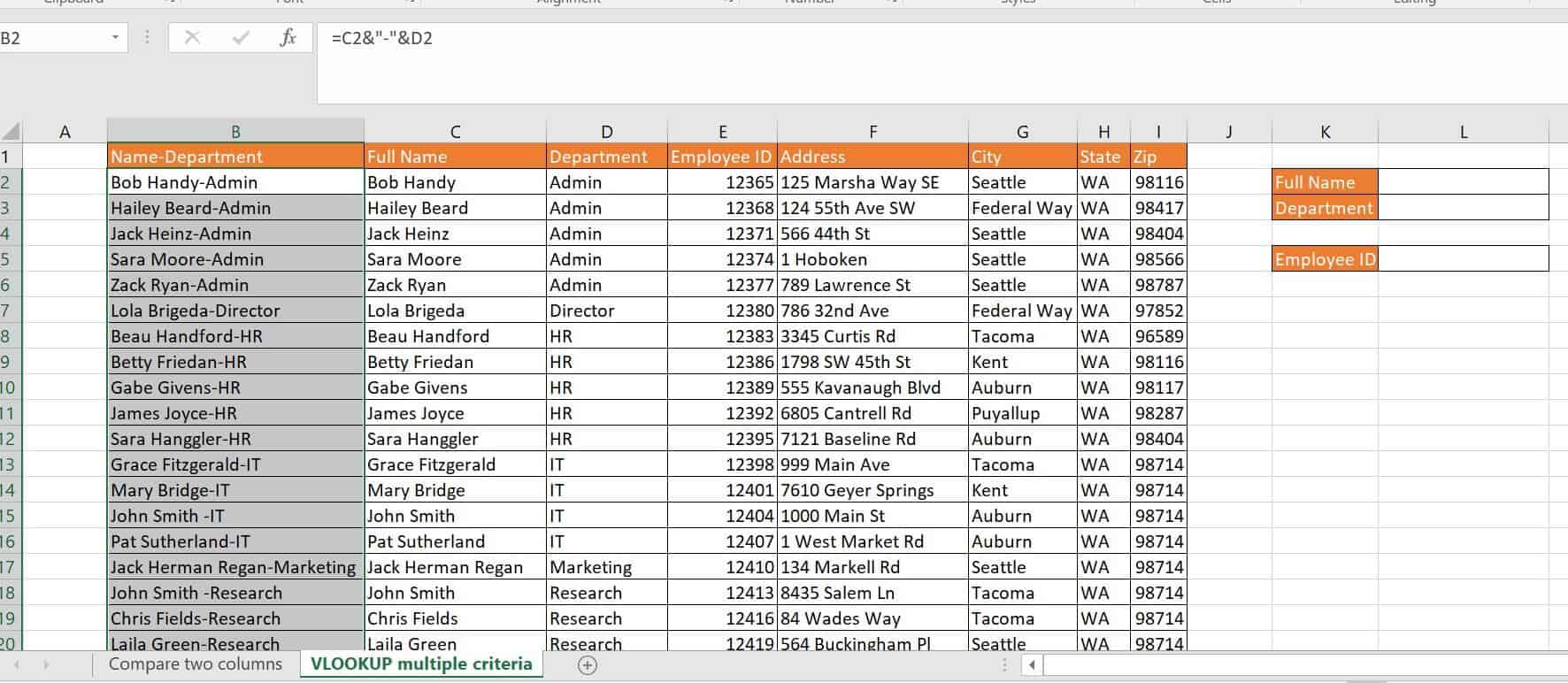
This worksheet lists staff members, their respective departments, and other pertinent details. However, there are two John Smiths: one who works in Research and one who works in IT. To get the right John Smith for your lookup, you will need to make each John Smith unique in the first column of your table.
2. Keeping in mind the best practices of performing a lookup in Excel, insert a lookup box into your spreadsheet that is at least one column or row away from your database for your VLOOKUP formula.
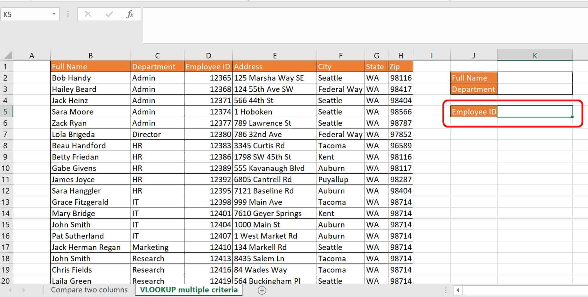
In the sample file, you’ll see additional boxes to input multiple reference data.
3. Select column B in your worksheet, insert a column to the left, and label it Name-Department.
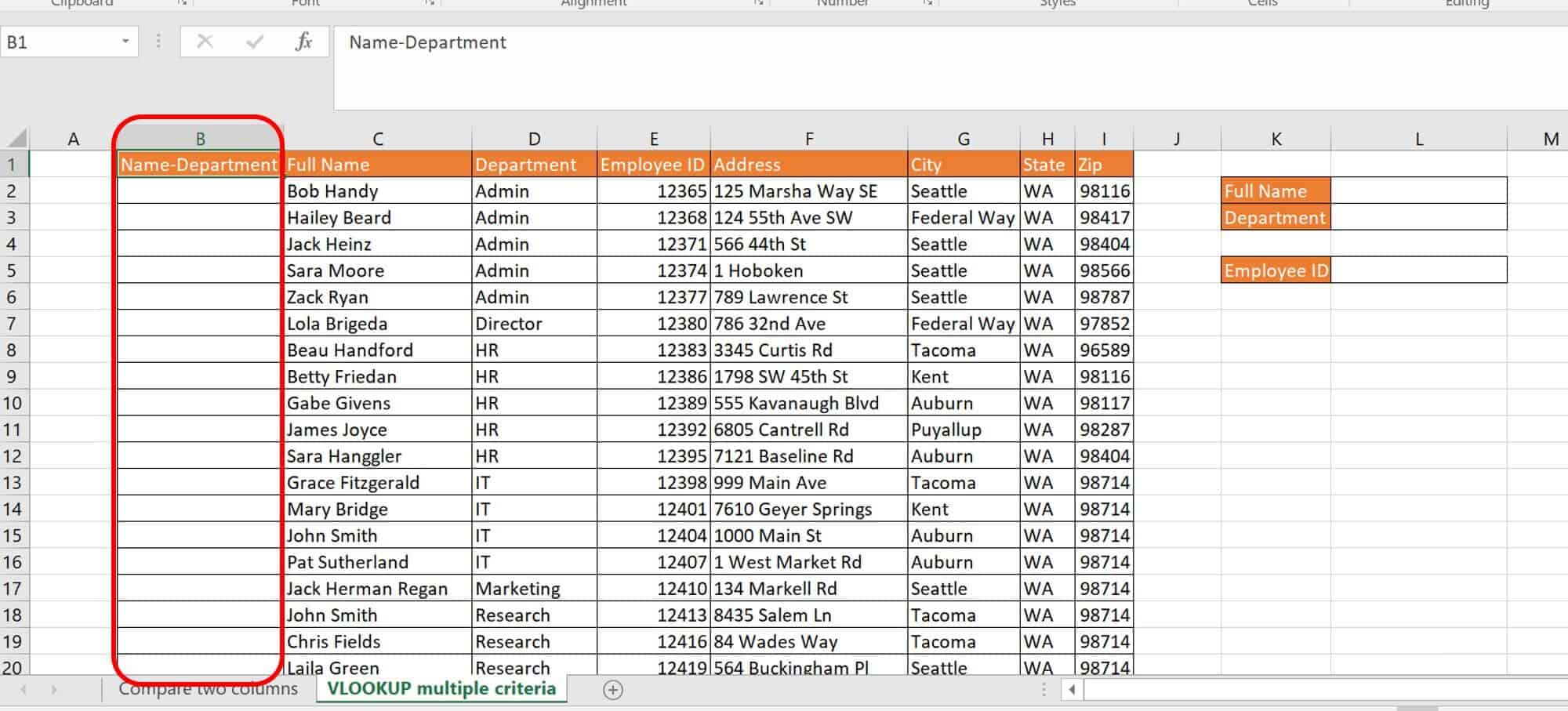
4. In cell B2, type in the following formula:
=C2&”-“&D2
This formula concatenates two cells’ information, cells C2 and D2 with a hyphen (-) in the middle. Click Enter on your keyboard.
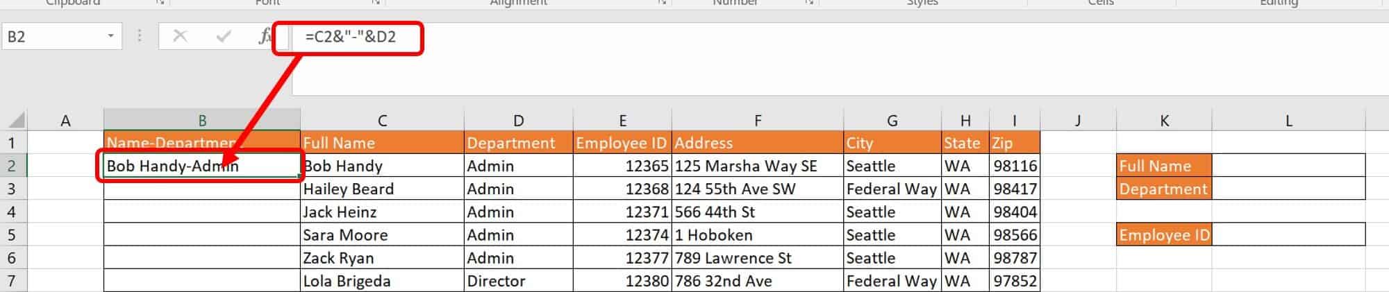
Now you have a unique value in your new cell B2.
5. Drag the formula down the length of column B in the table.
6. In cell L5, type in the following VLOOKUP formula:
=VLOOKUP(L2&L3,B1:I25,4,FALSE)
You can also use this identical formula:
=VLOOKUP(CONCATENATE(L2,"-",L3),B1:I25,4,FALSE)
Breaking down this formula:
Argument | Value | Meaning |
Lookup_Value | L2&”-“&L3 OR CONCATENATE(L2,”-“,L3) | The two lookup arguments separated by a dash “-“. Each ampersand (&) is a concatenation symbol that tells Excel to combine the values. The second option for this is to spell out the CONCATENATE function. |
Table_array | B1:I25 | The data table range. |
Col_index_num | 4 | The column where Excel needs to go to retrieve the return value. |
[Range_lookup] | FALSE | FALSE denotes an exact lookup return value. |
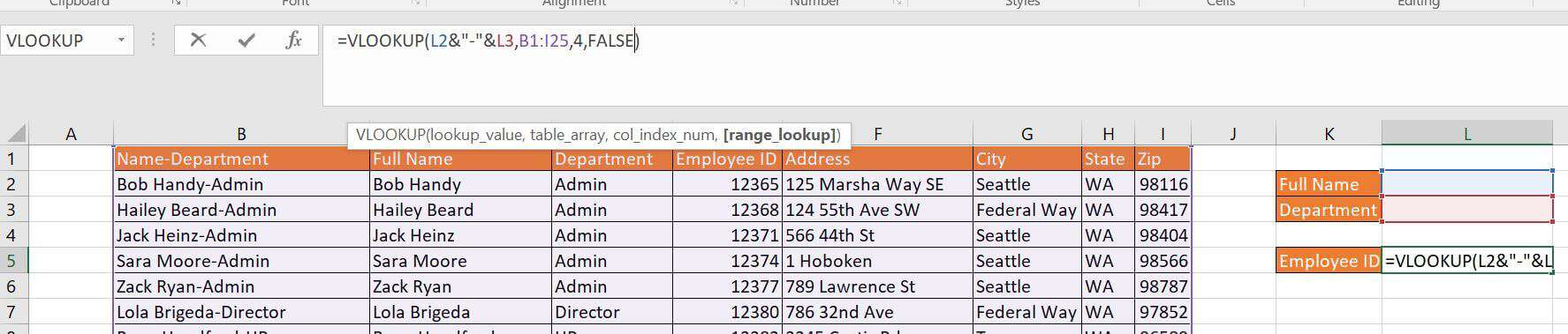
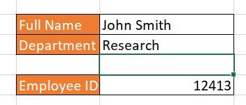
7. Using the formula and lookup boxes to find his Employee ID, type John Smith in cell L2 and Research in cell L3 to get the employee ID for the correct John Smith.
You can perform this for more than two criteria as long as the “helper” column has unique data in the rows, and it matches what you are searching for in the VLOOKUP formula. Concatenation is a great way to account for multiple-string search criteria.
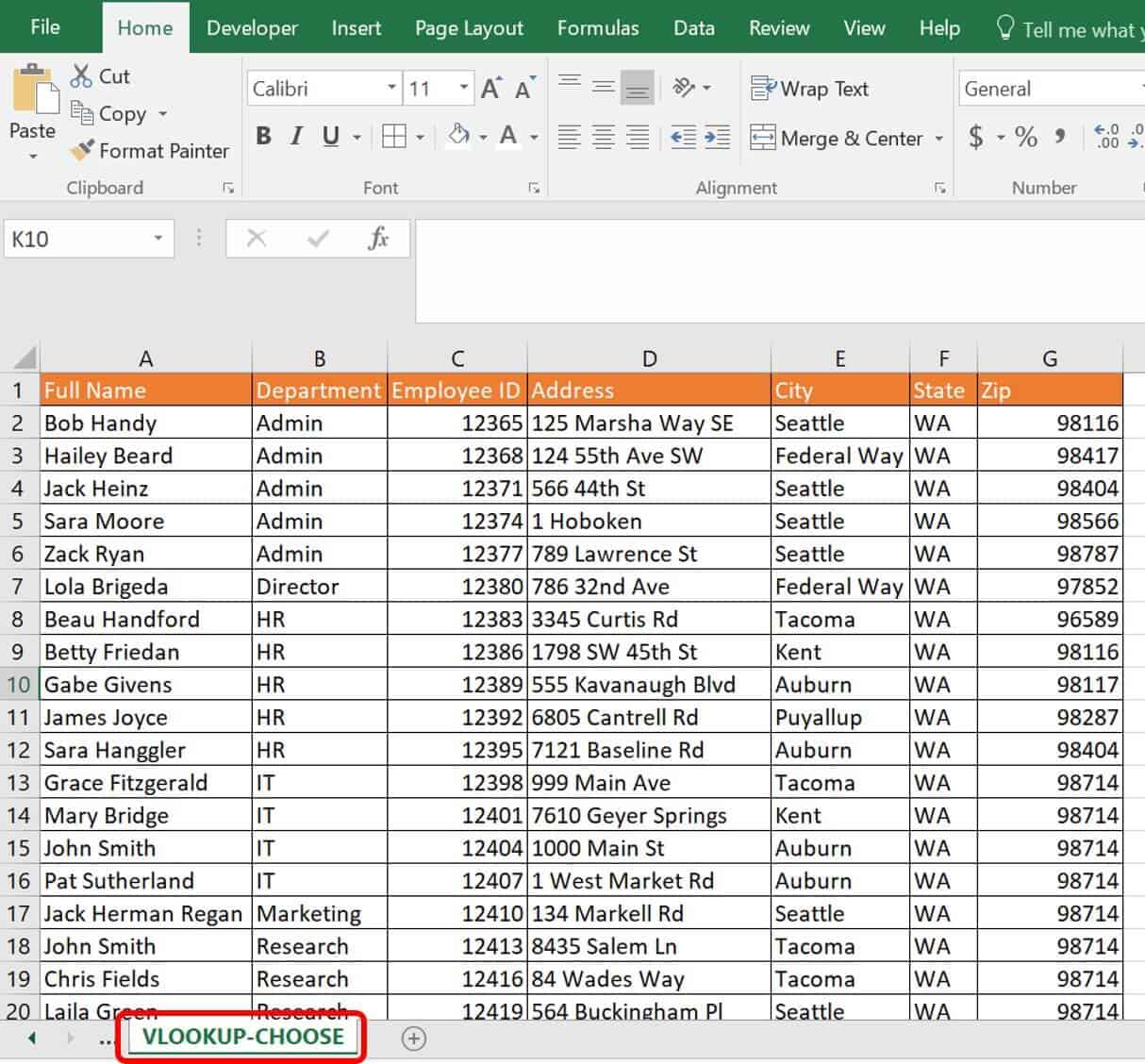
How to Combine VLOOKUP and CHOOSE with Multiple Criteria
A different method to perform the same multiple-criteria lookup is to use a CHOOSE function nested inside your VLOOKUP formula. There are two criteria, the Full Name and the Department, that you can use to get the correct Employee ID. Since there may be multiple people with the same name, use both criteria to identify the correct person.
To perform a VLOOKUP and CHOOSE combination with multiple criteria, follow these steps.
1. Click on the VLOOKUP-CHOOSE worksheet tab in the VLOOKUP Advanced Sample file .
2. Insert lookup boxes in the same manner as you did in the exercise for a VLOOKUP with multiple criteria, spacing them at least one column or row away from the database.
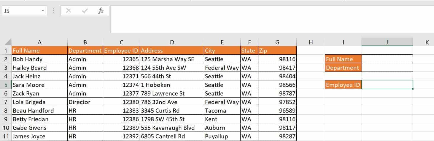
3. Type the following formula into cell J5:
=VLOOKUP(J2&"-"&J3,CHOOSE({1,2},A2:A25&"-"&B2:B25,C2:C25),2, FALSE)
Breaking down this formula, enter the first argument of the VLOOKUP:
Argument | Value | Meaning |
Lookup_Value | J2&"-"&J3 OR CONCATENATE(J2,”-“,J3) | The two lookup arguments separated by a dash “-“. Each ampersand (&) is a concatenation symbol that tells Excel to combine the values. The second option for this is the CONCATENATE function spelled out. |
The CHOOSE function fulfills the second argument of the VLOOKUP formula, defining the database where reference data resides. The CHOOSE formula:
CHOOSE({1,2},A2:A25&"-"&B2:B25,C2:C25)
CHOOSE creates a temporary table when you add an array to it, which is a slightly different use for the CHOOSE function than normal.
Argument | Value | Meaning |
Index_num | {1,2} | This array, surrounded by {}, is more than one specified index number, evaluating for both possibilities in the formula. |
Value1 |
| This value creates a table of two columns: A2:A25-B2:B25 (concatenated together) and C2:C25. |
Continuing the VLOOKUP, here are the last two arguments:
Argument | Value | Meaning |
Col_index_num | 2 | The column for pulling the return — in this case, C2:C25. |
[range_lookup] | FALSE | FALSE specifies an exact match is returned. |
4. Enter the formula, then click Enter on your keyboard.
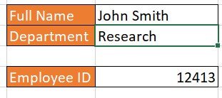
5. Type John Smith into the Full Name box, cell J2, and Research into the Department box, cell J3, and click Enter on your keyboard.
VLOOKUP-CHOOSE is one of the slowest formulas to calculate in comparison to other formulas in this guide. This possible drain on your computing power is due to the nature of Excel having to check every cell more than once for the required criteria.
How to Perform VLOOKUP for Multiple Criteria Using the Array Formula
Adding an array to your normal formulas essentially directs Excel to create and perform functions on virtual data. This is data you will not see in any cell but is still calculated. An array operates on a range of values and is enclosed in curly brackets { } that populate when you type Ctrl+Shift+Enter on the keyboard. Manually typing in these curly brackets on the outside of the formula will not create an array formula.
Additionally, arrays can use operators. Two such operators are:
- The AND operator (*); TRUE is returned if all conditions return as TRUE.
- The OR operator (+); TRUE is returned if any of the conditions return as TRUE.
SUM, MAX, and AVERAGE are three functions that work the same when combined with VLOOKUP for multiple criteria.
Follow these steps to perform VLOOKUP for multiple criteria with the SUM function.
1. Click on the VLOOKUP-Arrays worksheet tab in the VLOOKUP advanced sample file .
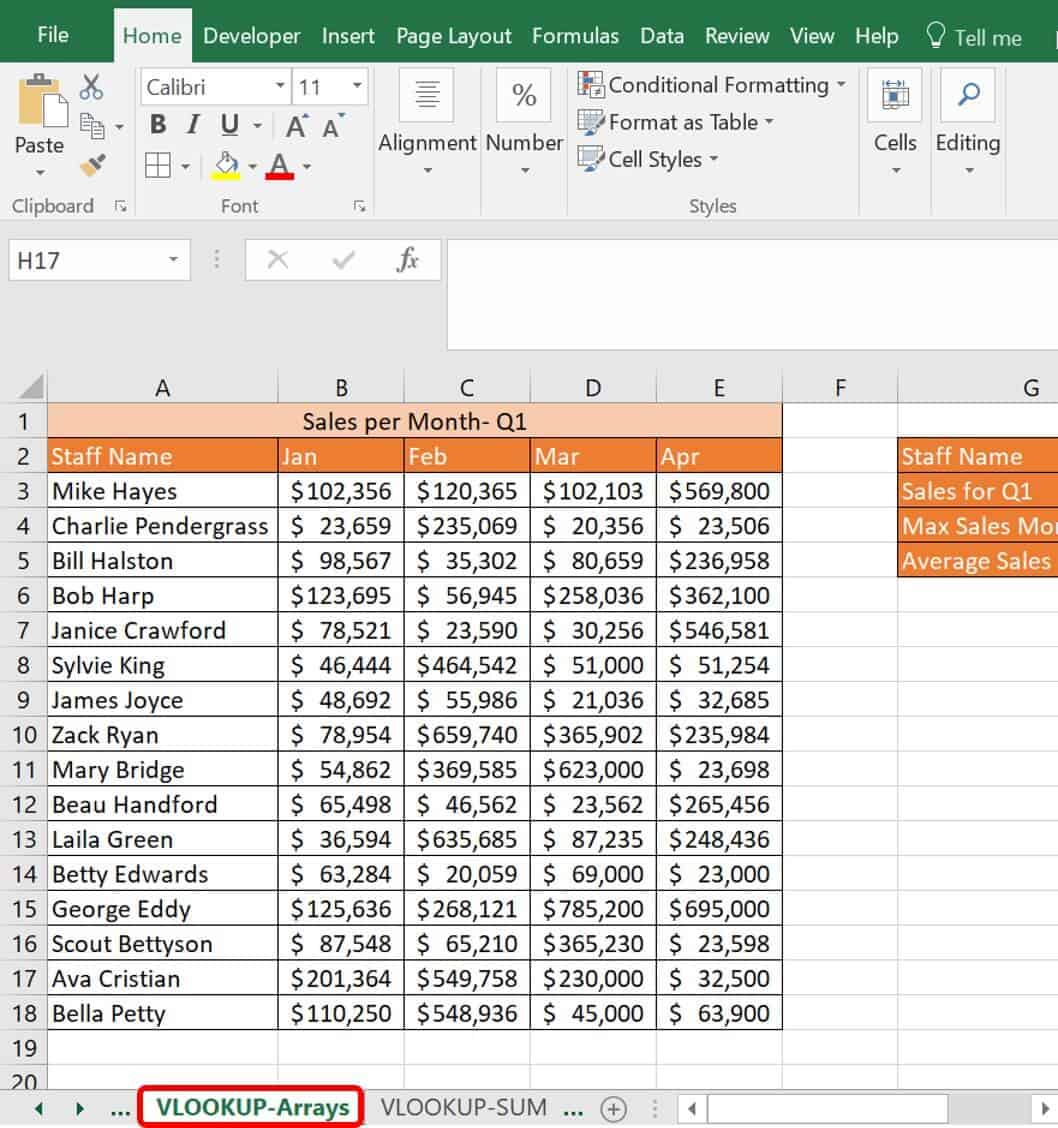
This worksheet has data about a sales staff and how much each employee sold in the first quarter. Use combined VLOOKUP formulas to find the SUM for each person. You could easily add another column to this worksheet to sum up the columns, but if you wanted to do this calculation on another worksheet or workbook with thousands of lines of data, it gets complicated. A combined formula is the most prudent route. Since this covers multiple criteria, you will add an array.
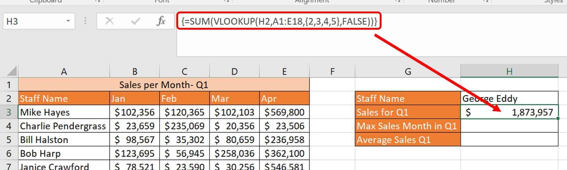
2. Type the SUM-VLOOKUP formula in cell H3:
=SUM(VLOOKUP(H2,A1:E18,{2,3,4,5},FALSE))
3. Click Ctrl+Shift+Enter on your keyboard to add the curly brackets:
{=SUM(VLOOKUP(H2,A1:E18,{2,3,4,5},FALSE))}
Breaking down the formula for the VLOOKUP:
Argument | Value | Meaning |
Lookup_value | H2 | The reference value Excel is looking for in the data table. |
Table_array | A1:E18 | The data table Excel reviews to find the reference value. |
Col_index_num | {2,3,4} | The columns Excel moves over to report back. Manually type the curly brackets { } in this portion of the formula. |
[Range_lookup] | FALSE | Requires an exact match. |
The formula is then wrapped in a SUM function, since the return is multiple values in an array. Without the extra SUM function, the VLOOKUP would return only the left-most value in the array: $125,636.
For George Eddy, Excel virtually recognizes that you are referring to several columns (columns 2, 3, 4, and 5) as your col_index_num and performs the requested SUM function. The return for the innermost function (the VLOOKUP) is: {$125,636, $268,121, $785,200, $695,000}. This return is virtual, and Excel returns the sum of $1,873,957 in cell H3.
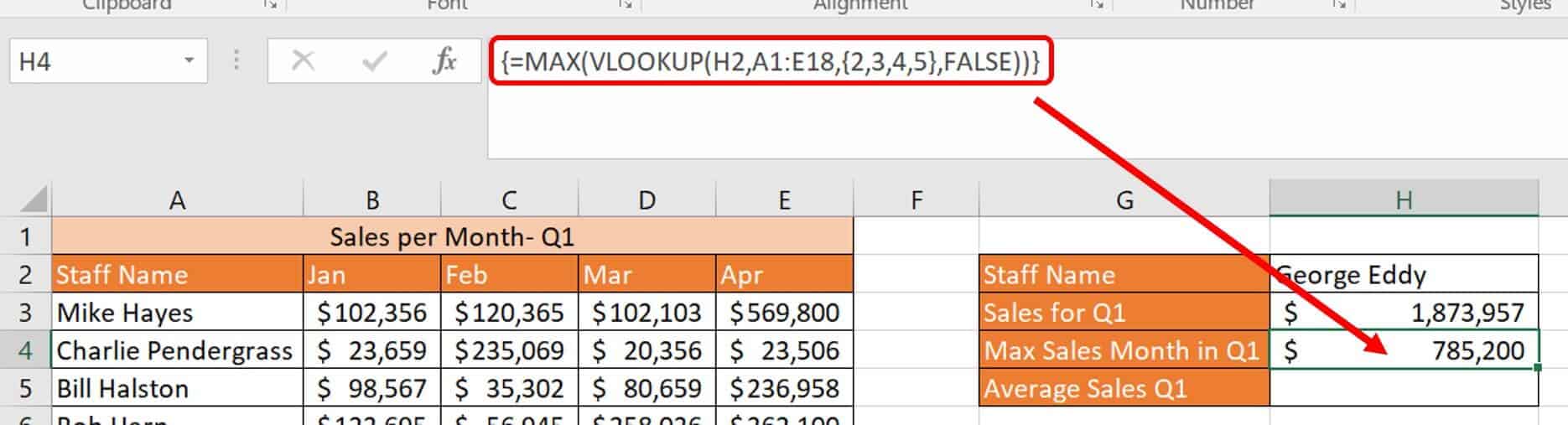
Follow these steps to perform VLOOKUP for multiple criteria with the MAX function.
- On the same worksheet tab, type the following formula in cell H4:
=MAX(VLOOKUP(H2,A1:E18,{2,3,4,5},FALSE)) - Click Ctrl+Shift+Enter on the keyboard to add the array around this formula.
Breaking down the formula for the VLOOKUP:
Argument | Value | Meaning |
Lookup_value | H2 | The reference value Excel is looking for in the data table. |
Table_array | A1:E18 | The data table Excel reviews to find the reference value. |
Col_index_num | {2,3,4} | The columns Excel moves over to report back. Manually type the curly brackets { } in this portion of the formula. |
[Range_lookup] | FALSE | Requires an exact match. |
The formula is wrapped in a MAX function, since it returns multiple values in an array. If you did not wrap the formula in the MAX function, the array would return data in the first column of the VLOOKUP, regardless of how many values requested in the array.
For George Eddy, Excel virtually recognizes that you are referring to several columns (columns 2, 3, 4, and 5) as your col_index_num and performs the requested function MAX. The return for the innermost function (the VLOOKUP) is then: {$125,636, $268,121, $785,200, $695,000}. This return is virtual, and Excel returns the max of these values, $785,200, in cell H4.
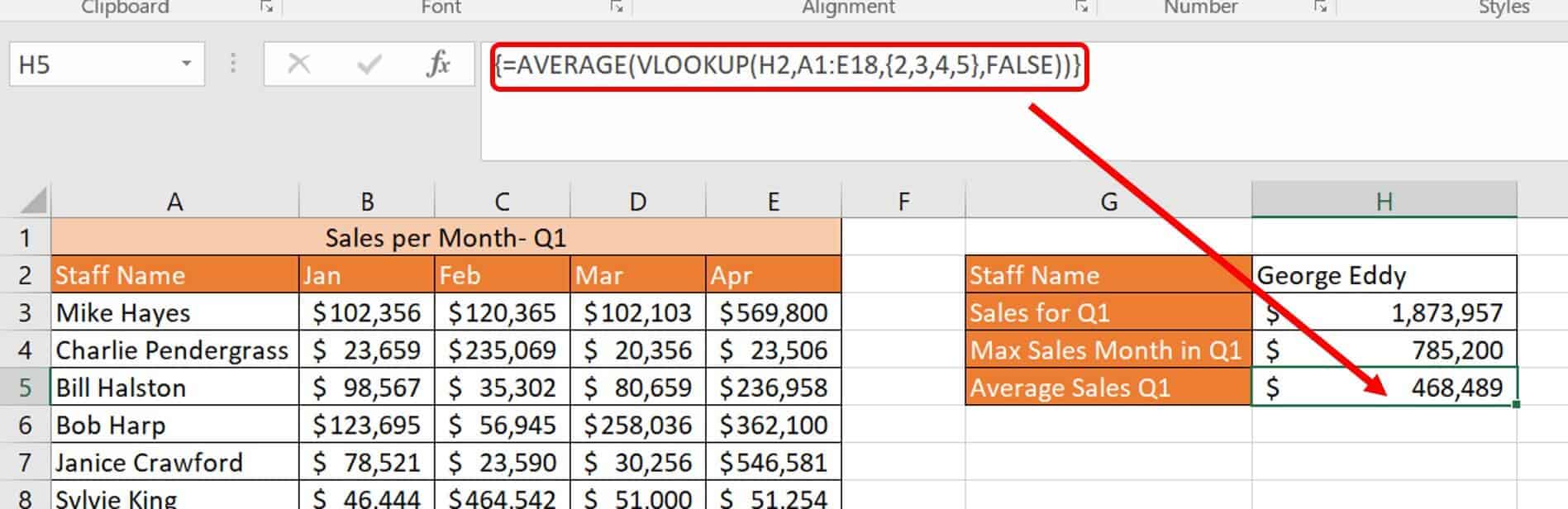
Follow these steps to perform VLOOKUP for multiple criteria with the AVERAGE function.
- On the same worksheet tab, type the following in cell H5:
=AVERAGE(VLOOKUP(H2,A1:E18,{2,3,4,5},FALSE)) - Click Ctrl+Shift+Enter on the keyboard to add the array around this formula.
Breaking down this formula for the VLOOKUP:
Argument | Value | Meaning |
Lookup_value | H2 | The reference value Excel is looking for in the data table. |
Table_array | A1:E18 | The data table Excel reviews to find the reference value. |
Col_index_num | {2,3,4} | The columns Excel moves over to report back. Manually type the curly brackets { } in this portion of the formula. |
[Range_lookup] | FALSE | Requires an exact match. |
The formula is then wrapped in an AVERAGE function, since the return is multiple values in an array. If you did not wrap the formula in the AVERAGE function, the array would return data in the first column of the VLOOKUP, regardless of how many values requested in the array.
For George Eddy, Excel virtually recognizes that you are referring to several columns (columns 2, 3, 4, and 5) as the col_index_num and performs the requested function AVERAGE. The return for the innermost function (the VLOOKUP) is then: {$125,636, $268,121, $785,200, $695,000}. This return is virtual, and Excel returns the average of these values, $469,489, in cell H5.
One neat trick when working with arrays: Click the F9 key while selecting a portion of the formula. You’ll get a bird’s-eye view of what is going on in the array virtually.
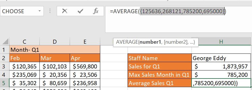
Here, the VLOOKUP formula alone is selected, and clicking F9 on the keyboard calculates the selected portion of the formula. Clicking the Esc key sets the formula back to normal.
Multiple VLOOKUPs Combined with SUM
Combining one VLOOKUP with another function is pretty straightforward, as demonstrated in the previous section. You can also combine multiple VLOOKUPs with another function for more complex results.
Follow these steps to perform multiple VLOOKUPs combined with SUM.
1. Click on the VLOOKUP-SUM worksheet tab.
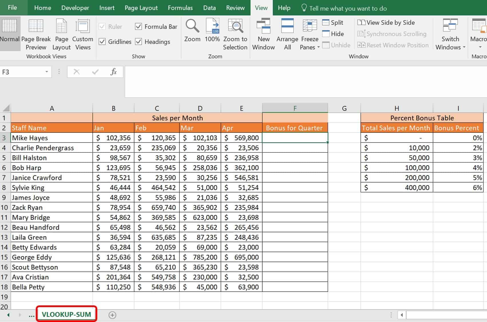
This worksheet tab has sales staff and their sales per month for the first quarter. You are tasked with figuring out their bonuses, which are calculated monthly and based on a monthly threshold in the Percent Bonus Table. When a salesperson meets the $10,000 threshold for the month, their bonus percentage escalates. Prior to $10,000 in sales, they do not receive a bonus.
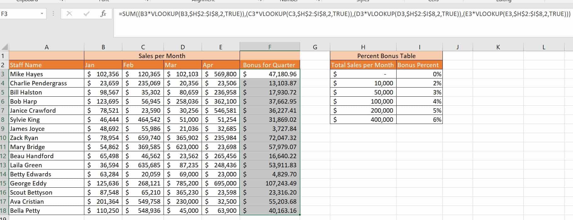
2. Type the following formula in your first cell, F3:
=SUM((B3*VLOOKUP(B3,$H$2:$I$8,2,TRUE)),(C3*VLOOKUP(C3,$H$2:$I$8,2,TRUE)),(D3*VLOOKUP(D3,$H$2:$I$8,2,TRUE)),(E3*VLOOKUP(E3,$H$2:$I$8,2,TRUE)))
The VLOOKUPs determine each monthly bonus virtually by performing the lookup in the table and returning the percent earned multiplied by that month’s total. Then the four months are summed to determine the quarterly bonus. All the VLOOKUPs work in the same way.
Breaking down the first one:
Argument | Value | Meaning |
Lookup_value | B3 | The reference value Excel is looking for in the data table. |
Table_array | H2:I8 | The data table Excel reviews to find the reference value. |
Col_index_num | 2 | The columns Excel moves over to report back. |
[Range_lookup] | TRUE | Requires an approximate match. |
The virtual return of this VLOOKUP is 0.04 since the amount for January is over $100,000. The 0.04 is then multiplied by the original amount (*B3). The SUM formula is next wrapped around the multiple VLOOKUPs, using the return from each as inputs. From there, the formula virtually becomes:
=SUM((4094.24),(4814.6),(4084.12),(34188))
3. Click and drag the formula down through the table, from cell F3 to F18.
How to Perform VLOOKUP Combined with SUMIF
SUMIF is an Excel function that sums that values in a specified range. The syntax for SUMIF is: SUMIF=(range,criteria,[sum_range]). The difference between SUM and SUMIF is that SUMIF performs the summation only if the values meet specific criteria.
Follow these steps to perform a multiple VLOOKUP combined with SUMIF.
1. Click the VLOOKUP – SUMIF worksheet tab in the VLOOKUP Advanced Sample file.
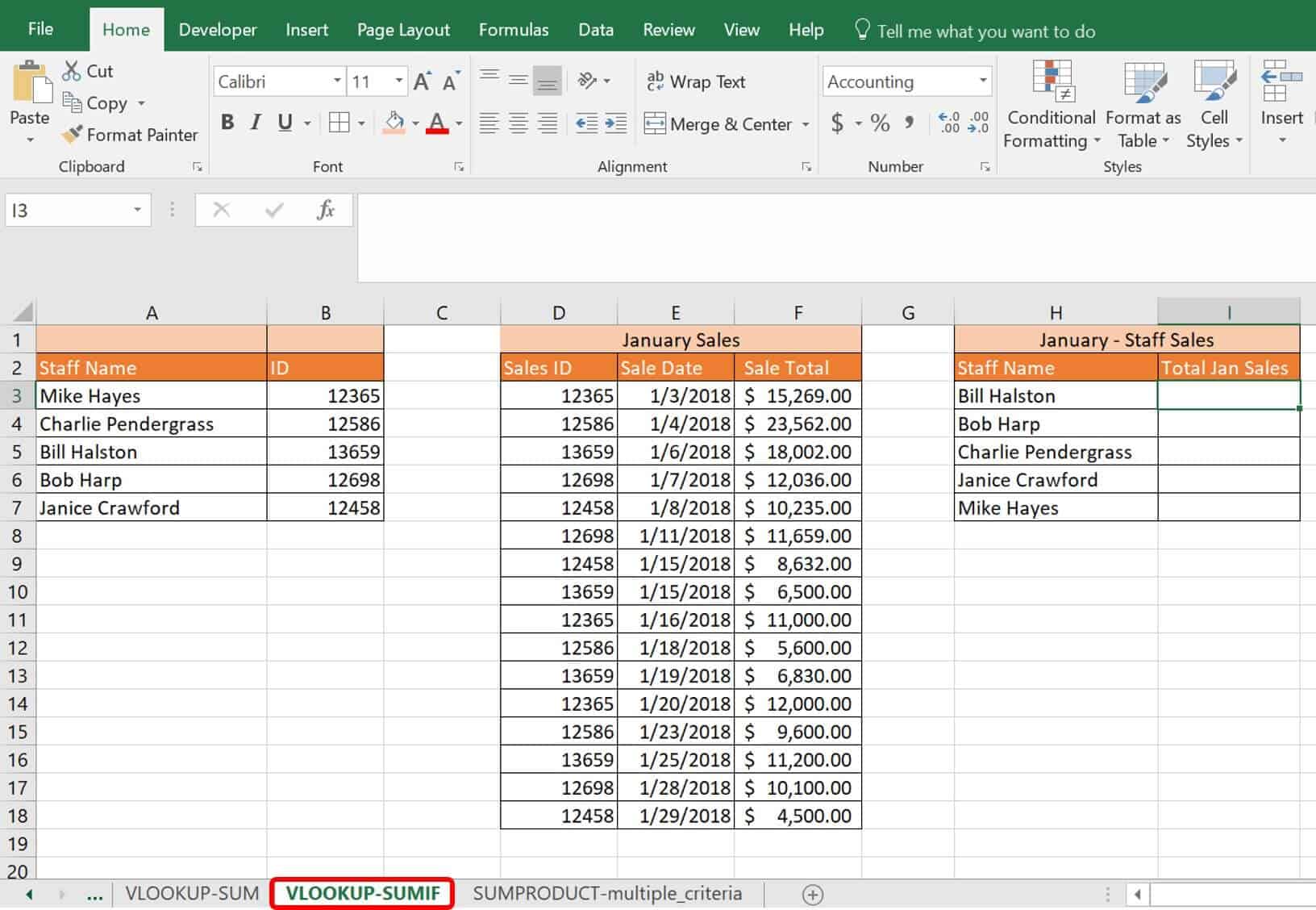
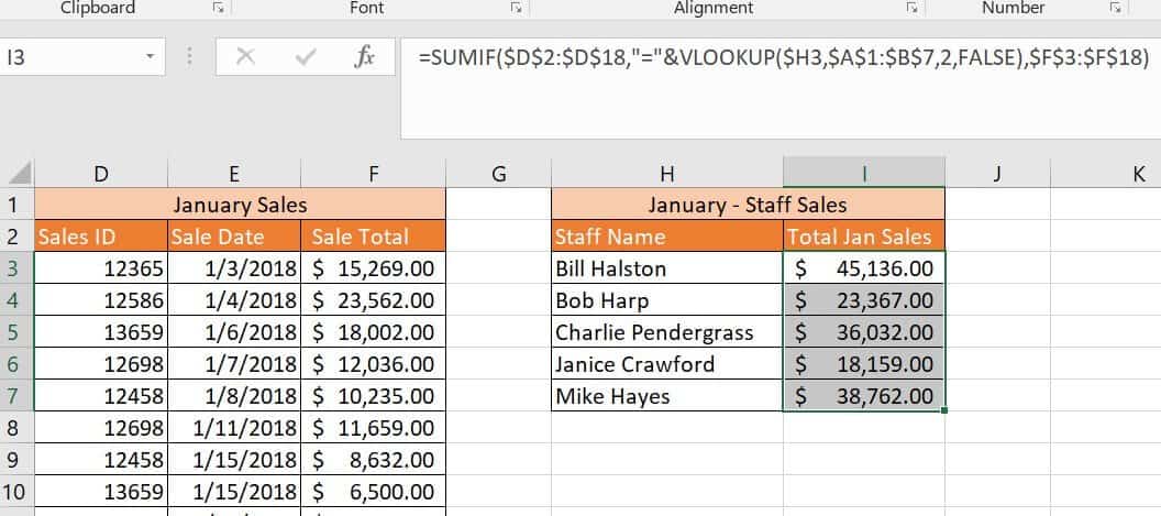
This worksheet has two tables: the staff names with corresponding ID numbers, and January sales data. Unfortunately, the January sales data is listed by staff ID, and you need the data matched to their name and totaled for their monthly sales total to credit the right staff member.
2. Type the following formula in cell I3:
=SUMIF($D$2:$D$18,"="&VLOOKUP($H3,$A$1:$B$7,2,FALSE),$F$3:$F$18)
Breaking down this formula, the VLOOKUP is performed first:
Argument | Value | Meaning |
Lookup_value | H3 | The reference value Excel is looking for in the data table. |
Table_array | A1:B7 | The data table Excel reviews to find the reference value. |
Col_index_num | 2 | The columns Excel moves over to report back. |
[Range_lookup] | FALSE | Requires an exact match. |
The virtual result of the VLOOKUP is 13659. Excel virtually returns Bill Halston’s ID number. Wrapped in a SUMIF function, you have left:
=SUMIF($D$2:$D$18,"="&13659,$F$3:$F$18)
Breaking down the SUMIF function:
Argument | Value | Meaning |
range | D2:D18 | The range that Excel is searching to find the criteria, which is the Sales ID column. |
criteria | “=”&VLOOKUP return | Tells Excel that your VLOOKUP return (13659) is part of a formula to look for, and creates a universal formula you can drag into other cells. |
[sum_range] | F3:F18 | The actual data that is summed, based on what is defined by the criteria. |
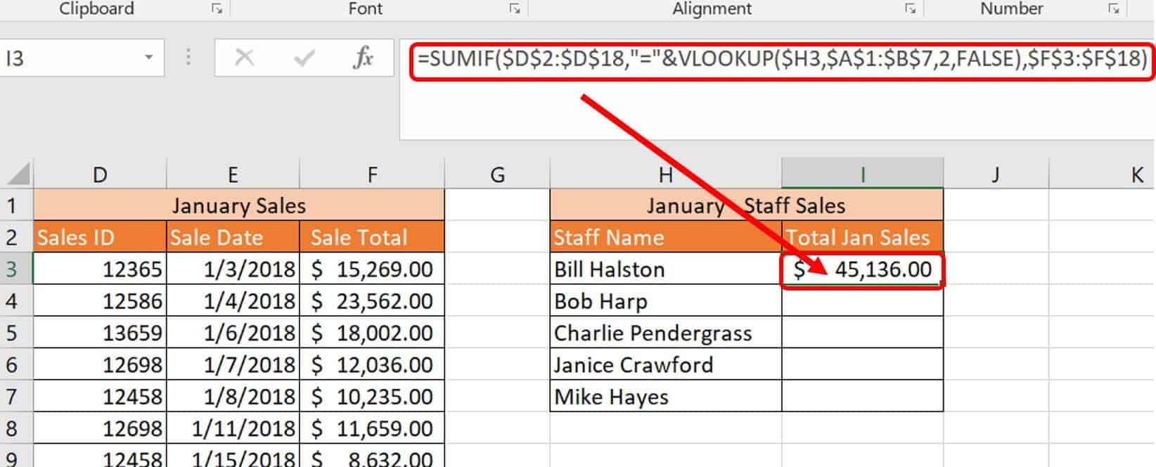
3. Once you enter the formula, click and drag cell I3 down through cell I7 to add the formulas for your staff.
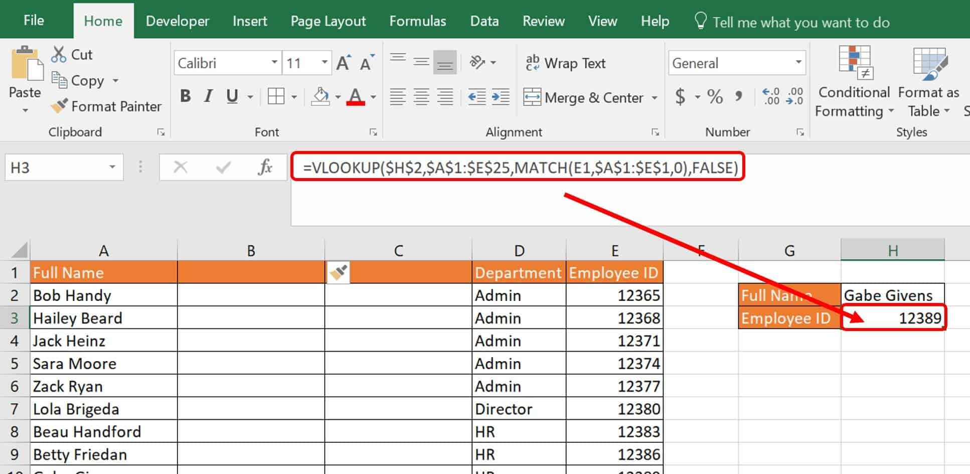
VLOOKUP and MATCH Combined for Updates
One of the most onerous problems with VLOOKUP is when users make changes (columns are added, deleted, or simply moved) to a workbook and you must rewrite all the formulas. This issue is frustrating and time-consuming. VLOOKUP on its own does not respond well to change. However, combining VLOOKUP with MATCH shifts the story. Instead of dealing with a #REF error, add a MATCH formula as the col_index_ref in the VLOOKUP; it can respond dynamically.
Follow these steps to combine VLOOKUP and MATCH to prevent change errors.
1. Click on the VLOOKUP-MATCH worksheet tab in the VLOOKUP Advanced Sample file .
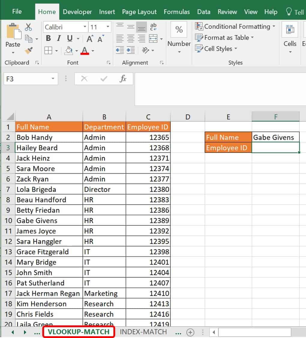
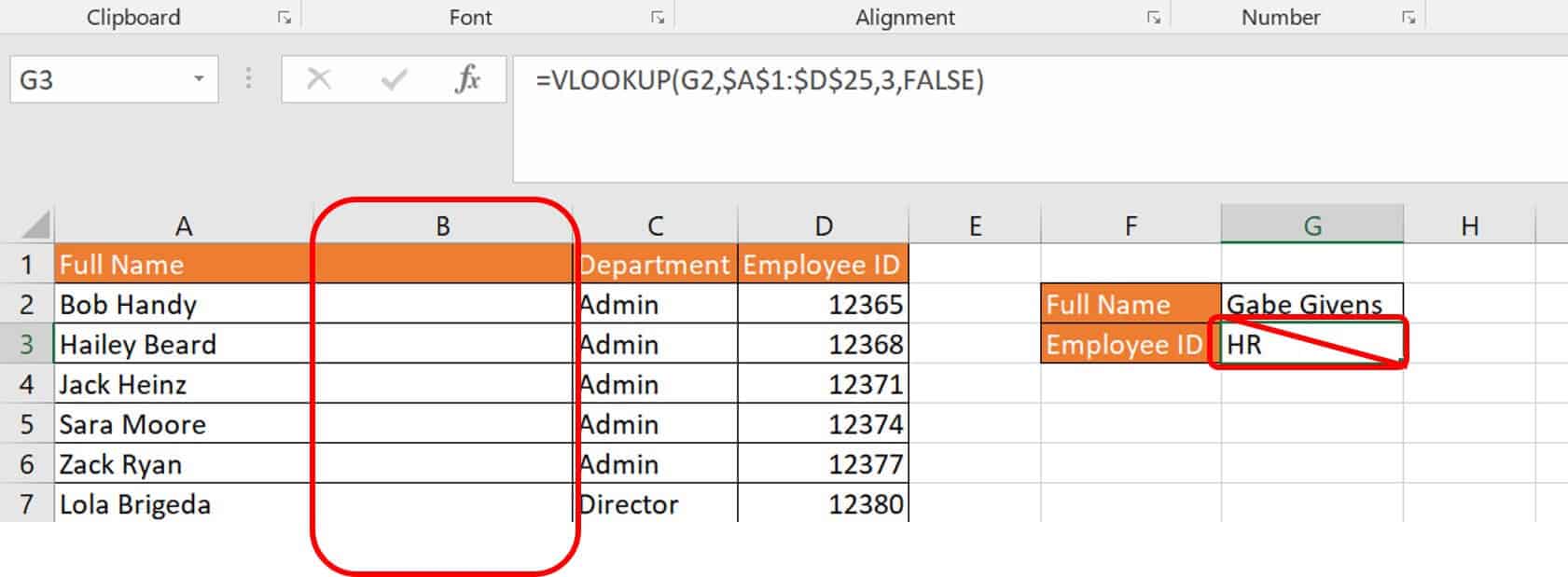
This is a simple worksheet that lists staff’s full names, departments, and employee IDs. You would normally add a simple VLOOKUP formula in cell F3 to return the employee ID when given the staff full name, such as the following:
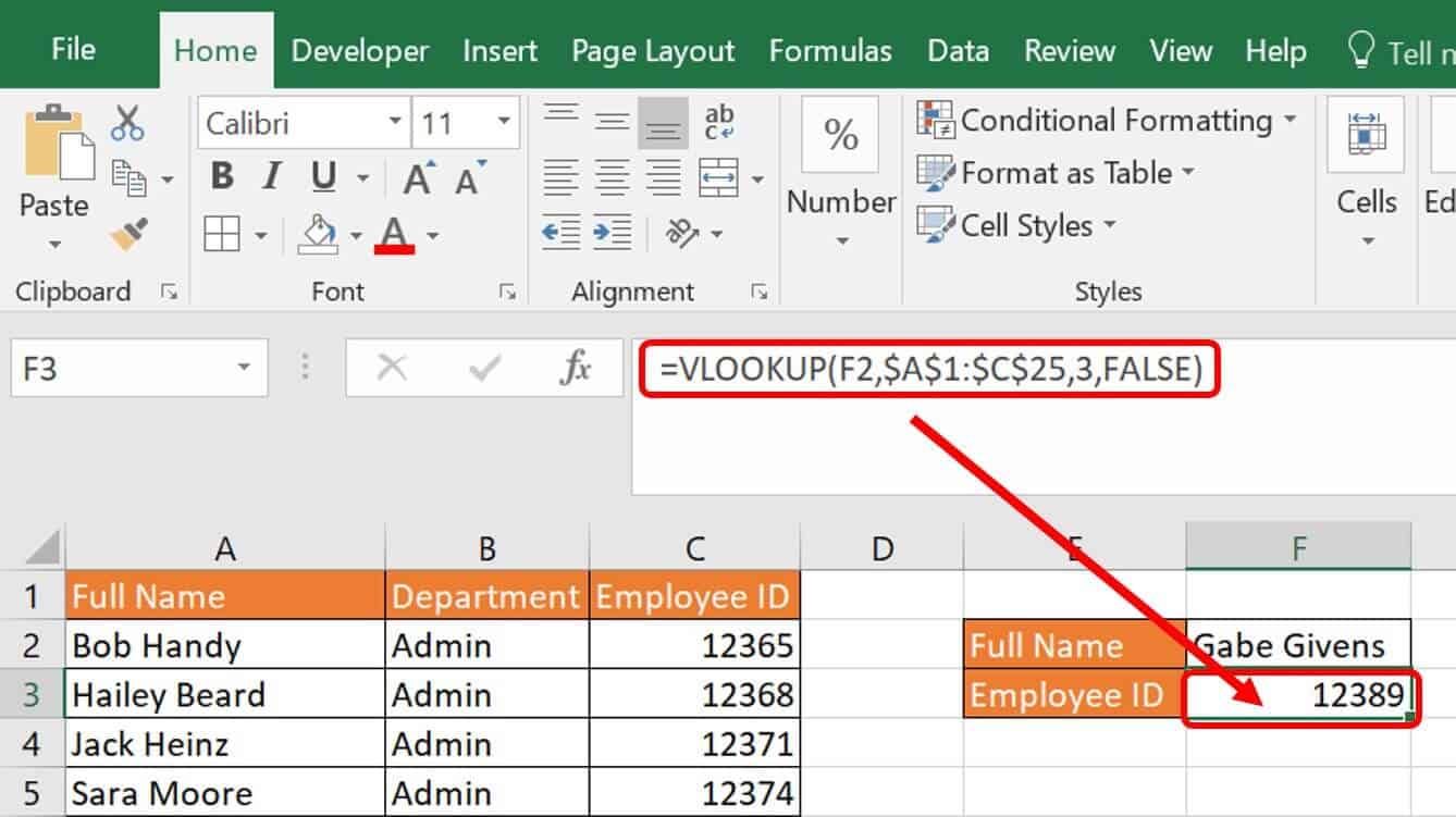
However, when you add a column for more data, it returns the wrong data.
2. In cell G3, type the following formula:
=VLOOKUP($G$2,$A$1:$D$25,MATCH(D1,$A$1:$D$1,0),FALSE)
The difference here is that the col_index_num is the MATCH formula. The syntax for MATCH is the following:
=MATCH(lookup_value,lookup_array,[match_type])
Breaking down this formula:
Argument | Value | Meaning |
Lookup_value | D1 | The reference value, the employee ID, which is the column you want returned. |
Lookup_array | A1:D1 | The column header row, telling the formula to look for the reference value wherever it’s located in the table. |
[match_type] | 0 | The value 0 is an exact match. |
Why Index-Match Is Better than VLOOKUP
When working with Excel, it is important to learn other formulas for performing the same task. Some functions take up considerably more computing power than others, especially if there are many lines of data in your database. With some newer updates to Microsoft products, more system resources are required than ever before. Features such as excessive or conditional formatting, unused styles, shapes, and certain formulas take up a lot of memory and can cause workbooks to run slowly and even crash.
Lookup functions are notorious for taking up a lot of memory. One method of decreasing this computing power is to design lookups that reference a limited range and not the whole column of data if it’s not needed. Another method is to use other formulas that perform the same type of task. INDEX-MATCH is a combination formula that can replace your VLOOKUP that uses less memory because you are pointing the formula to precisely where the formula should look for data.
INDEX is a function that returns a table value based on its position within that table and is a lookup/reference function that you can use as part of a formula. In INDEX, you define the table, the exact row, and the exact column locations. The syntax is:
=INDEX(table,row_number,column_number)
INDEX is useful because it can return strings, numbers, and dates.
MATCH is also a lookup/reference function in Excel that you can use in combination with other formulas or on its own. MATCH looks for the value in your specified array and returns its location. The syntax for MATCH is:
=MATCH(lookup_value, lookup_array,[match_type])
The match_type is optional, which is why it is in brackets [ ]. Possible values of match_type are 1, 0, and -1. The default value is 1; it’s the largest value less than or equal to the value specified. A match_type of 0 returns the first value equal to the value specified (lookup_value). A match_type of -1 returns a value that is greater than or equal to the specified value (lookup_value). For match_types 1 and -1, you should sort the array.
For example, on the following column, if you typed in the MATCH formula:
=MATCH(A6,A:A,0)
Excel would return 6 since you specified Zack Ryan’s cell. Instead of the value in the cell, Excel assumes that your data range is an array and returns the cell’s location.
How to Use INDEX-MATCH with Multiple Criteria
When using INDEX-MATCH instead of VLOOKUP for multiple criteria, you have several options. Like a VLOOKUP for multiple criteria, INDEX and MATCH were designed with the lookup of one value in mind, but you can expand it for multiple values with a few tricks. What remains the same in any lookup function is that there needs to be a unique value to look up. Your options to write into this formula are:
- Use a helper column: Adding a data column to your database that concatenates two columns’ worth of data gives you a better chance of getting unique data to start from. If you use this, ensure the data typed in manually matches it. For instance, if you are looking for salary information for Tom Jones, and there are multiple Tom Jones in your company, you may want to combine names with birthdates or employee numbers to create unique values in the helper column account for multiple criteria being considered. INDEX-MATCH does not require that your lookup_value reside in the left-most column, so you can add the helper column anywhere in your data table.
Most Excel experts tend to look down on the helper column. Their mentality is that you should be able to neatly get your data from one column to another with multiple nested formulas and virtual data, minimizing the need for extra visual data. However, there are two issues with this attitude. First, when you are learning to master Excel, that visual data is a tremendous help. Second, you may actually save computing power with helper columns and data already present. With data calculated step-wise in different columns, Excel does not work as hard when you open a workbook as it does with formulas that do everything in one. - Concatenate criteria in your formula: Instead of making a helper column, your formula should specify two different criteria that are unique columns in the data table. Using CHOOSE with an array instead of your normal defined data table provides virtual columns of criteria for your formula to choose from.
- Add an array into the lookup formula: The following is an example of how to do this using an INDEX-MATCH combined formula.
Follow these steps to perform an INDEX-MATCH with multiple criteria.
1. Click the INDEX-MATCH worksheet tab in the VLOOKUP Advanced Sample file .
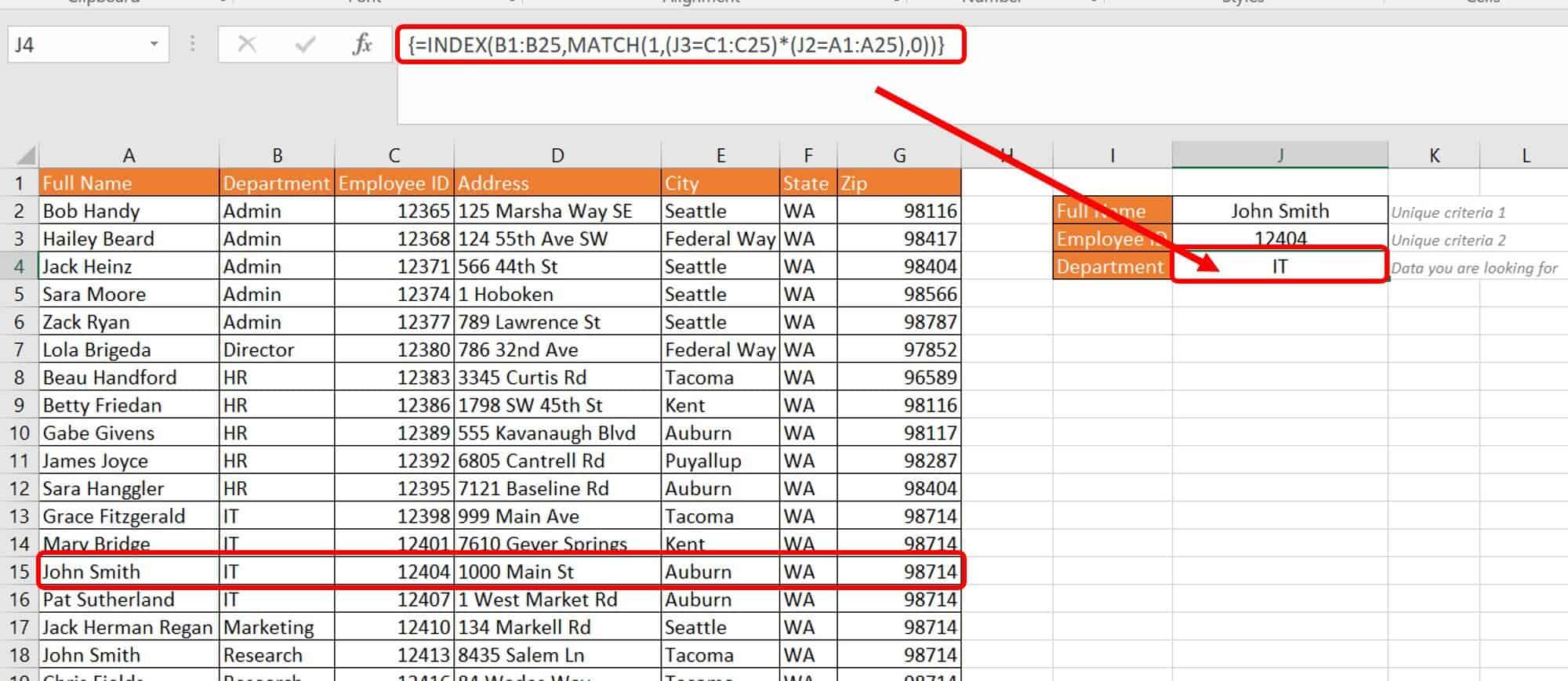
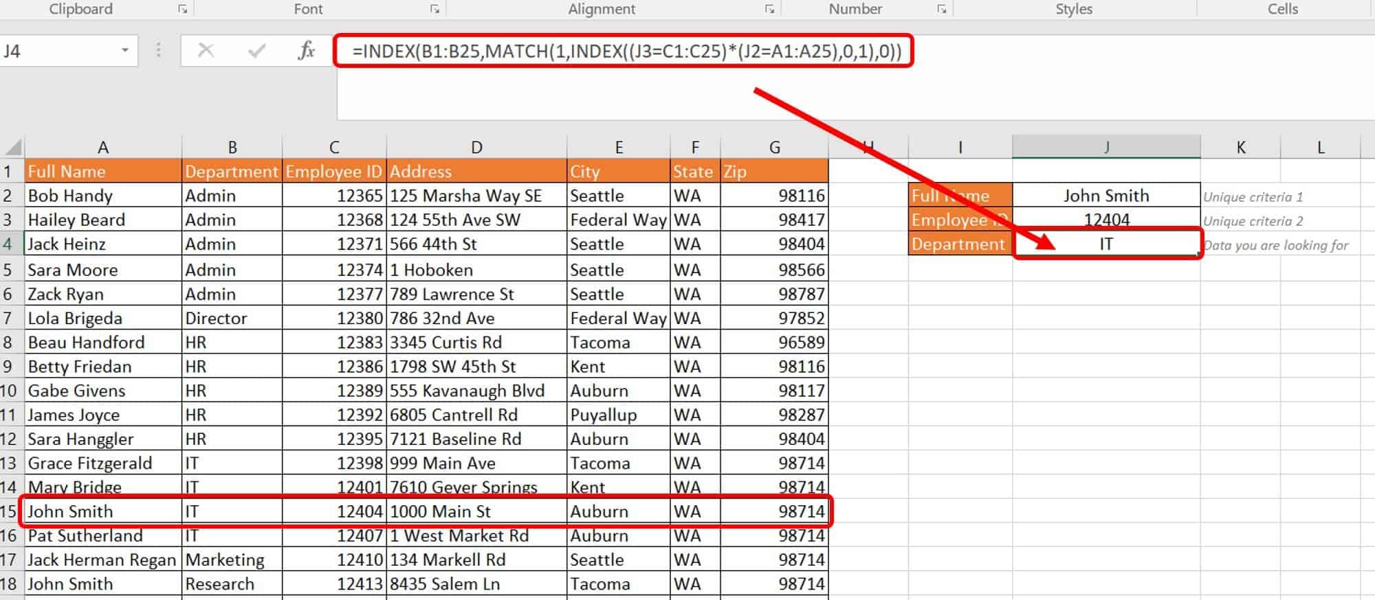
Much like the VLOOKUP tutorial, the INDEX-MATCH tutorial is set up to pull information from the datasheet. You’ll see multiple personnel with the same name. To differentiate them and get the department for a specific person, you need unique information for them — in this case, their full name and their employee ID.
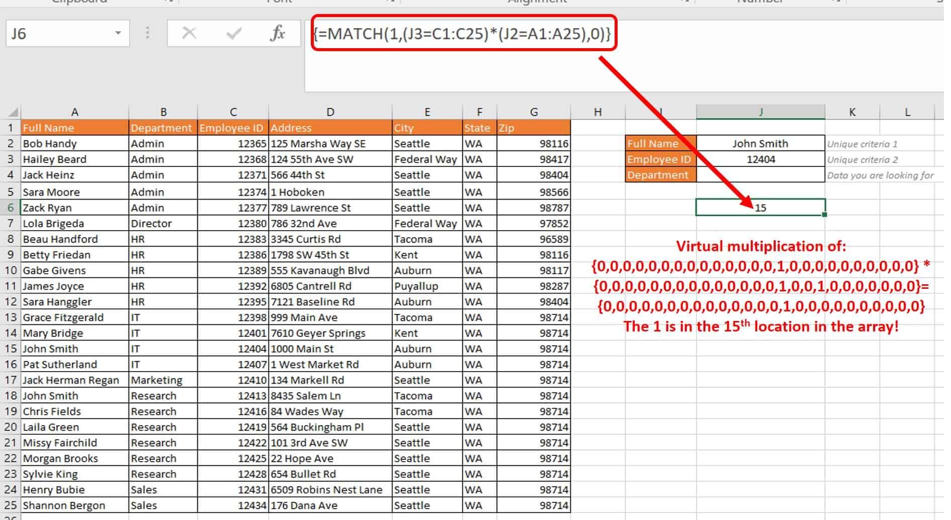
2. Type the following formula into cell J4:
=INDEX(B1:B25,MATCH(1,(J3=C1:C25)*(J2=A1:A25),0))
3. On your keyboard, click Ctrl+Shift+Enter to add an array around the formula so it looks like this:
{=INDEX(B1:B25,MATCH(1,(J3=C1:C25)*(J2=A1:A25),0))}
You cannot manually add curly brackets { } for an array in this formula.
Breaking down this formula, begin with the internal MATCH:
Argument | Value | Meaning |
Lookup_value | 1 | The value that the MATCH is trying to find. |
Lookup_array |
| The lookup array compares the defined employee ID against all of the employee IDs in column C, as well as the defined full name against the other full names in column A. This comparison returns instances of virtual TRUE (1) and FALSE (0) in arrays. When the multiplication operator (*) is used between them, they multiply by each other’s arrays until there is only one match (a virtual 1 among 0). This 1 location is the returned value: |
[match_type] | 0 | This is an exact match. |
As an example, the MATCH formula itself is that which requires the array, or the Ctrl+Shift+Enter (curly brackets). This formula alone returns 15.
Wrapping this result in an INDEX formula makes it into a standard INDEX formula:
=INDEX(B1:B25,15)
Argument | Value | Meaning |
Reference/array | B1:B25 | The second column’s data. |
Row_num | 15/MATCH return | The MATCH return. |
Another option is a non-array version. Add another INDEX into the formula like this:
=INDEX(B1:B25,MATCH(1,INDEX((J3=C1:C25)*(J2=A1:A25),0,1),0))
How to Use a Lookup to Return Multiple Matches
One of the known problems with VLOOKUP is that it can return only one match per formula and per cell. If you are using VLOOKUP for simple matches, such as pulling a value out of a huge database, this may not be an issue. However, if you need to get all matching values, VLOOKUP is limiting. One consistent theme you will see throughout your Excel training is that there are multiple ways to accomplish the same return using different functions and function combinations.
You can add together other functions such as IF, SMALL, INDEX, ROW, COLUMN, IFERROR, ISNA, ISBLANK, and COUNTIF. In the preceding sections, we introduced you to array formulas. These functions, in combination with arrays, provide multiple matches. Each has its own purpose and combines well with LOOKUP formulas:
- IF: (logical_test, [value if true], [value if false]); evaluates the condition you set and returns one value if it is met, and another if it is not met.
- SMALL: (array,k); returns the k-th smallest value in the array; “k” is thousand.
- INDEX: (array, row_num, col_num); returns the array component based on the row and column specified.
- ROW: ([reference]); returns the row number.
- COLUMN: ([reference]); returns the column number.
- IFERROR: (value,value_if_error); checks the reference and replaces with what’s specified if error is found.
- ISNA: (value); checks for #N/A error and substitutes with value specified if found.
- ISBLANK: (value); checks the specified value and returns TRUE if blank and FALSE if not blank.
- COUNTIF: (range, criteria); defines the range of cells to check and counts them if they meet the specified criteria.
Follow these steps to perform a LOOKUP of multiple values and return the results in a column.
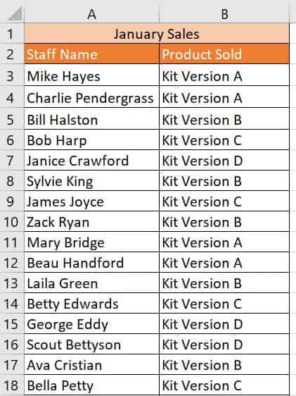
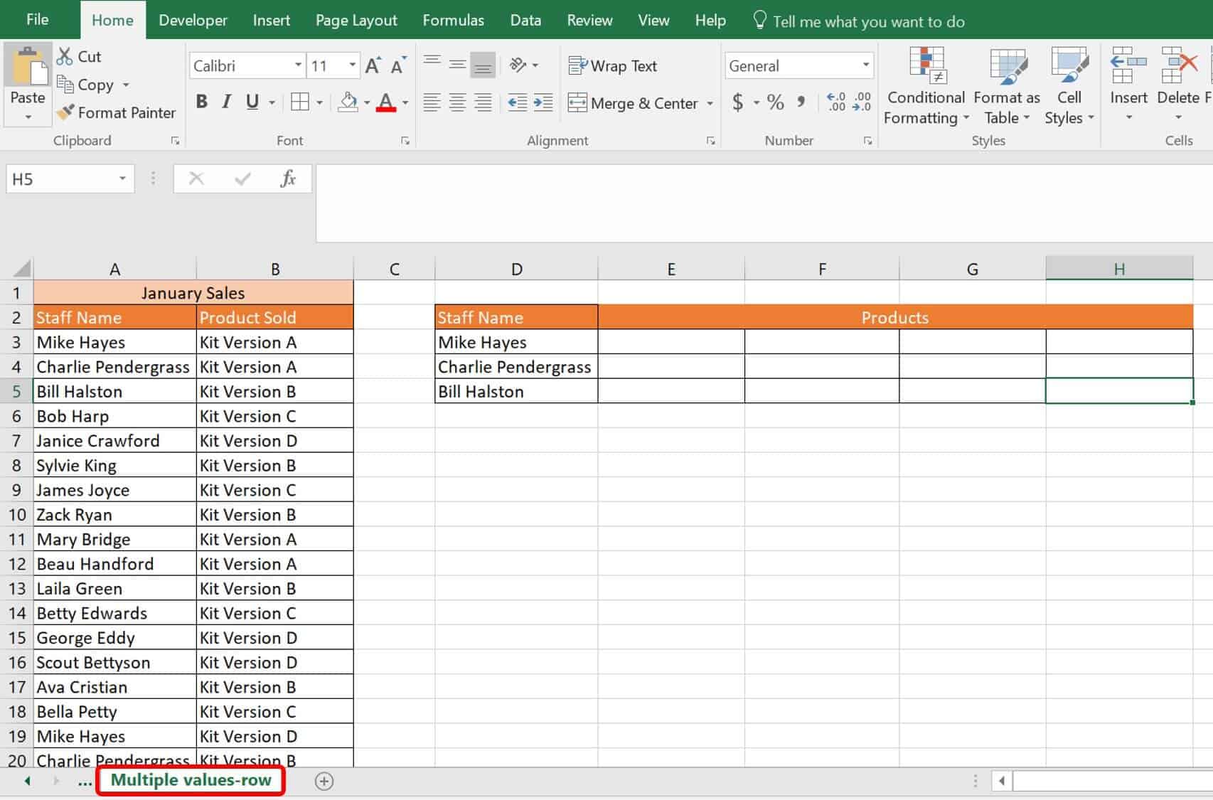
1. Click on the Multiple values-column worksheet tab in your VLOOKUP Advanced Sample file .
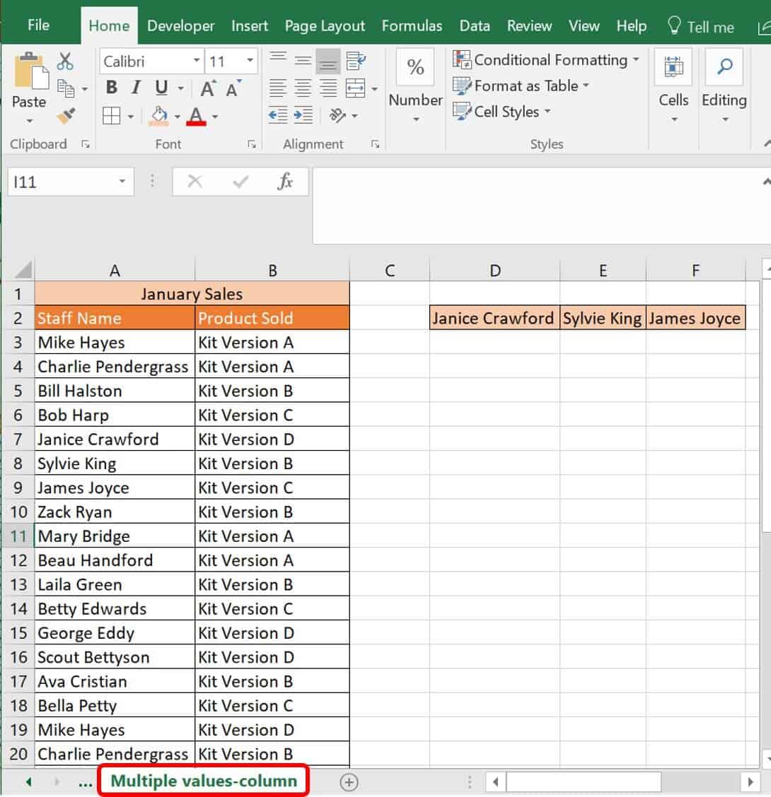
This file lists a unique row for your sales team and the products they sold in January. In this scenario, we are trying to find out which versions of the four kits (A, B, C, and/or D) were sold by three members of the sales staff.
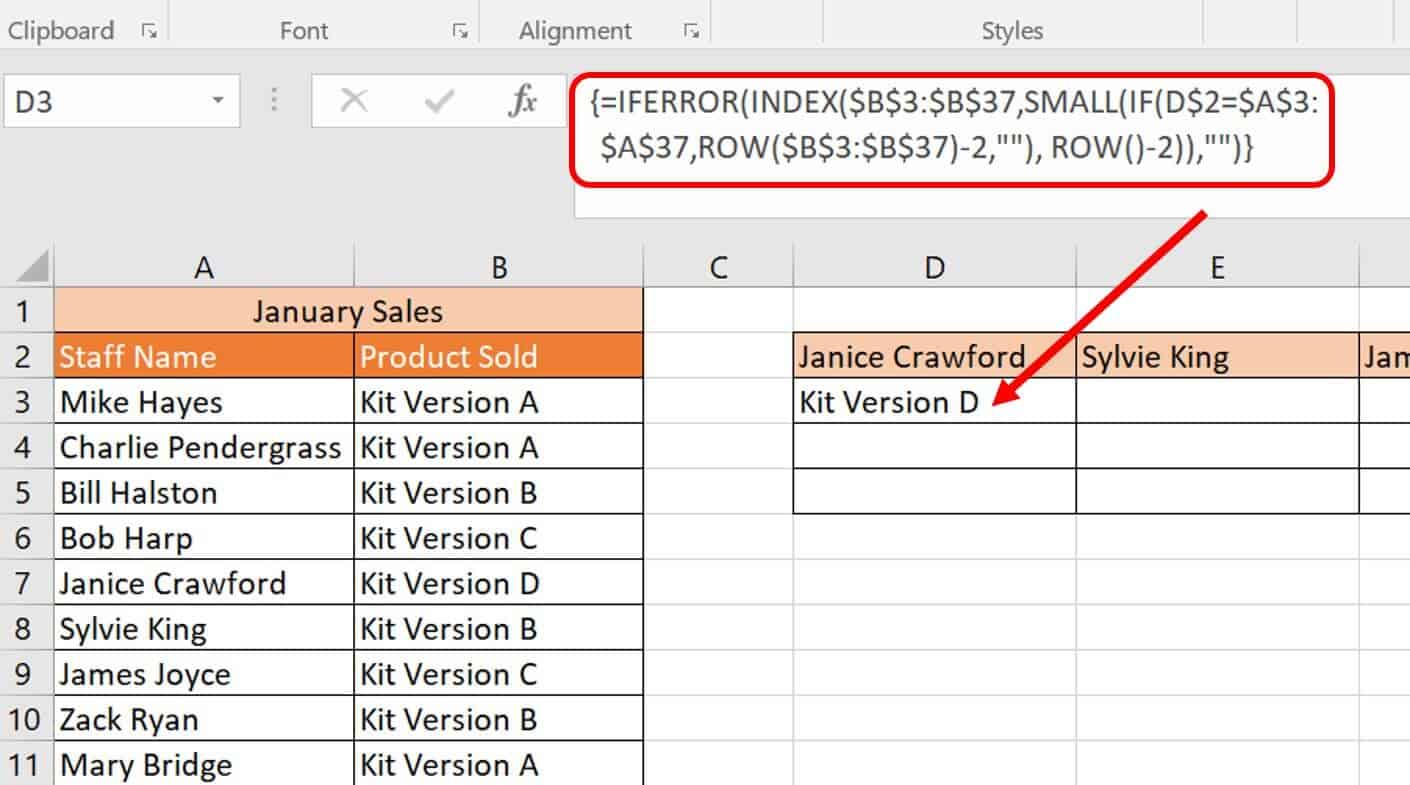
2. Type the following formula into cell D4 (under Janice Crawford):=IFERROR(INDEX($B$3:$B$37,SMALL(IF(D$2=$A$3:$A$37,ROW($B$3:$B$37)-2,""), ROW()-2)),"")
3. Click Ctrl+Shift+Enter on your keyboard to tell Excel this is an array formula.
Excel runs the IF formula found in the middle first. The syntax for IF, as shown above, is the following:=IF(logical_test, [value if true], [value if false])
This portion of the formula is the following:
IF(D$2=$A$3:$A$37,ROW($B$3:$B$37)-2,“”
This IF function compares the lookup value D2 with each value in the defined table range, A3:A37. In other words, the logical test is that the value in D2 (Janice Crawford) exists in each cell. If the function returns TRUE, then the row position is returned and two (2) is subtracted from it because of the row’s position in the table, which is two down from the top of the form with the headers in place.
If this is not true, the returned value is blank (“”). The absolute value signs ($) keep the column or row constant to account for copying/dragging it across and down a table. What is returned at this point is the virtual positions of the matches. The virtual return for this array function is: {"";"";"";"";5;"";"";"";"";"";"";"";"";"";"";"";"";"";"";"";21;"";"";"";"";"";"";"";"";"";"";"";33;"";""}
If you check this return, it shows that Janice Crawford appears in rows 5, 21, and 33 in the data table. (Note: These row numbers do not correspond to the row numbers in the worksheet because it accounts for the two rows used to create the table head.)
The SMALL function is calculated. This function analyzes and returns which matches should be returned in a cell. Right now, the SMALL formula look like this: SMALL({"";"";"";"";5;"";"";"";"";"";"";"";"";"";"";"";"";"";"";"";21;"";"";"";"";"";"";"";"";"";"";"";33;"";""},ROW()-2)
ROW()-2 is an incremental counter and places the results of the array in incremental order to not repeat. The virtual result of this function is 5.
What is left after the SMALL function has been calculated:
=IFERROR(INDEX(B3:B37,{5},””)
The INDEX is calculated next and returns the value of the array based upon its row number.
This return looks like this virtually:
IFERROR(“Kit Version D”),””)
Last is the IFERROR function, which ensures an error is not reported. An error could be reported if there were no values left to report in your column, and it reports either the product of your formula or a blank cell (“”).
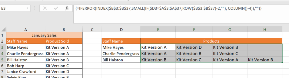
4. Select and drag cell D3 across through cell F3, and then all three cells D3 to F3 down for three to four cells (or how many sold products you think will return) to autofill the formula.
The result is what three sales team members sold in January. These are separate formulas in each cell, but the results are related to each other and therefore appear in a column-like list.
Follow these steps to perform a VLOOKUP of multiple values and return the results in a row.
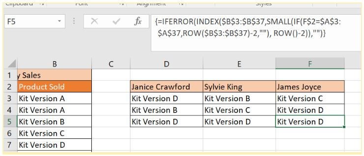
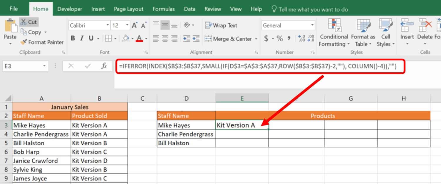
1. Click on the Multiple values-row worksheet tab in the sample file.
2. Type the following formula into cell E3:
=IFERROR(INDEX($B$3:$B$37,SMALL(IF(D$3=$A$3:$A$37,ROW($B$3:$B$37)-2,""), COLUMN()-4)),"")
3. Click Ctrl+Shift+Enter on your keyboard so Excel knows this is an array formula.
The first formula Excel runs is the IF formula in the middle. The syntax for IF, as shown above, is:
=IF(logical_test, [value if true], [value if false])
This portion of the formula is the follownig:
IF(D$3=$A$3:$A$37,ROW($B$3:$B$37)-2,“”
This IF function compares the lookup value D3 with each value in the defined table range, A3:A37. In other words, the logical test is that the value in D3 (Mike Hayes) exists in each cell. If the function returns TRUE, then the row position is returned and two (2) is subtracted from it because of where the row is positioned in the table. This row is positioned two down from the top of the form with the headers in place.
If this is not true, then the returned value is blank (“”). The absolute value signs ($) keep the column or row constant for copying/dragging it across and down your table. The virtual positions of the matches are returned. The virtual return for this array function is: {1;"";"";"";"";"";"";"";"";"";"";"";"";"";"";"";17;"";"";"";"";"";"";24;"";"";"";"";"";"";"";"";"";"";""}.
If you check this return, you’ll see that Mike Hayes appears in rows 1, 17, and 24 in the data table. (Note: These row numbers do not correspond to the row numbers in the worksheet because it accounts for the two rows used to create the table head.)
Next, Excel calculates the SMALL function, which analyzes the matches it should return in a cell. Right now, the SMALL formula looks like this: SMALL({1;"";"";"";"";"";"";"";"";"";"";"";"";"";"";"";17;"";"";"";"";"";"";24;"";"";"";"";"";"";"";"";"";"";""}, COLUMN()-4)
COLUMN()-4 is an incremental counter; it takes the results of your array and puts them in incremental order to not repeat. The virtual result of this function is 1.
What is left after the SMALL function has been calculated:
=IFERROR(INDEX(B3:B37,{1},””)
The INDEX is calculated next and returns the value of the array based upon its row number.
This return looks like this virtually:
IFERROR(“Kit Version A”),””)
The IFERROR function ensures that an error is not reported. An error could be reported if there were no values left to report in your column, so it reports either the product of your formula or a blank cell (“”).
4. Select and drag the cell E3 across through cell H3, and then all four cells E3 to H3 down and across for two cells (E5 through H5) to fill in the formula. Since Ctrl+Shift+Enter was performed for the first cell with the formula (E3), this will carry over to the other cells if you select and drag the formula.
Follow these steps to perform a LOOKUP of multiple matches from multiple conditions
1. Click on the Multiple matches-criteria worksheet tab.
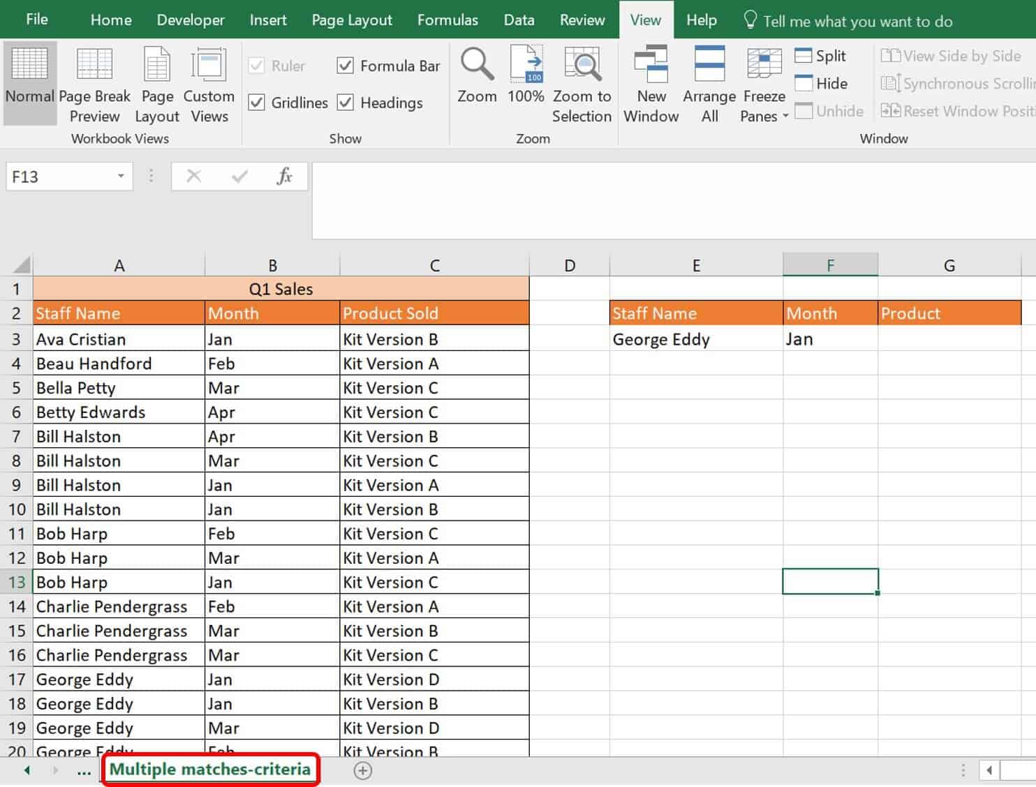
This worksheet tab shows the sales team and products sold for the first quarter. The formula you add is similar to that in the exercise for returning multiple values in a column, except you are returning multiple criteria in more than one column. The Month column is added to the lookup table. In this exercise, let’s determine what products George Eddy sold by month in the first quarter.
2. Type the following formula in cell G2:
=IFERROR(INDEX($C$3:$C$37, SMALL(IF(1=((--($E$3=$A$3:$A$37)) * (--($F$3=$B$3:$B$37))), ROW($C$3:$C$37)-2,""), ROW()-2)),"")
3. Click Ctrl+Shift+Enter on the keyboard. Next, click and drag the formula down three or four cells (G3, G4, G5, and G6) to add it to the cells beneath G2:
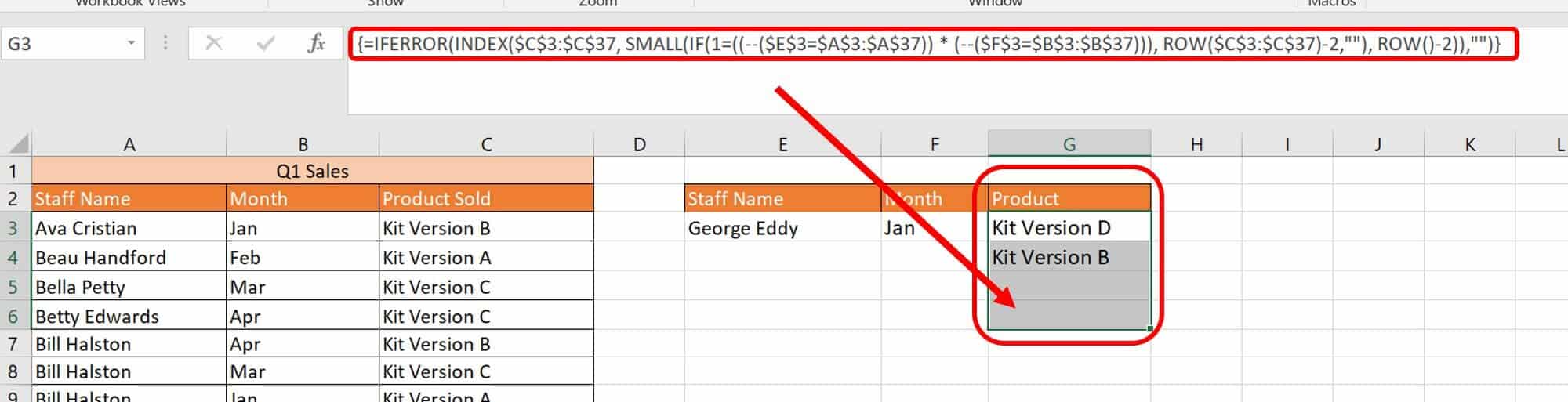
The result is the data in column form based on two criteria: the staff name and the month of sales.
This formula is different than the one in the Multiple values-column worksheet tab because you are using the AND (*) operator in the IF function to concatenate the two lookup criteria. The IF function in this formula is the following:
IF(1=((--($E$3=$A$3:$A$37)) * (--($F$3=$B$3:$B$37))), ROW($C$3:$C$37)-2,"")
Similar to results seen in the formulas above, the array formulas return either TRUE or FALSE for each array. In the first array condition, 1=((--($E$3=$A$3:$A$37) identifies TRUE/FALSE returns for the Staff Name of George Eddy. The -- in the formula is the same as multiplying the result by 1 (and can be replaced by 1). This information helps Excel push the results into numeric form. The second array condition is (--($F$3=$B$3:$B$37)), which looks for the month Jan. Overall, you are asking for both array conditions to be met. The result of this IF function is the following: {"";"";"";"";"";"";"";"";"";"";"";"";"";"";15;16;"";"";"";"";"";"";"";"";"";"";"";"";"";"";"";"";"";"";""}
How to Use SUMPRODUCT in a Lookup with Multiple Criteria
SUMPRODUCT is another function that you can use to perform a lookup. SUMPRODUCT is an Excel function that multiplies arrays and returns the sum of the products. The syntax for SUMPRODUCT is below:
SUMPRODUCT=(array1,[array2],[array3]…)
Follow these steps to perform a lookup with multiple criteria using SUMPRODUCT.
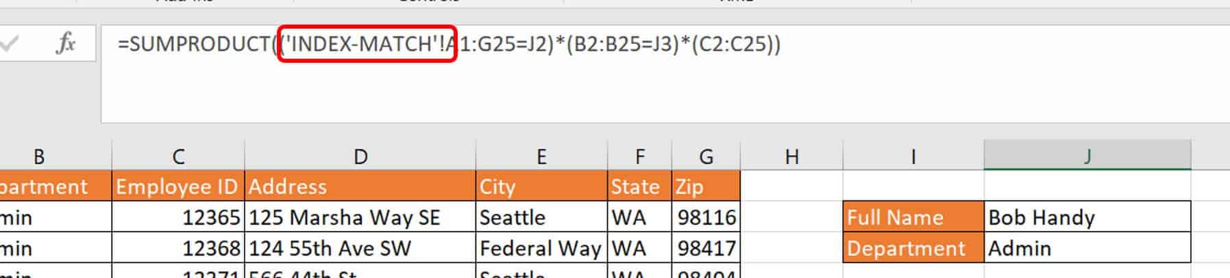
1. Click on the SUMPRODUCT-multiple_criteria worksheet tab in the VLOOKUP Advanced Sample file .
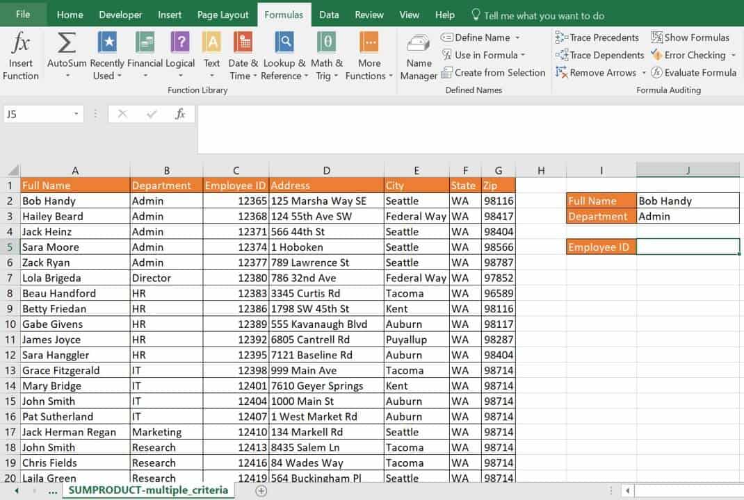
This worksheet tab has a portion of staff, contact information, department, and ID numbers. In this example, let’s use the criteria of Full Name and Department to look for an employee’s ID number.
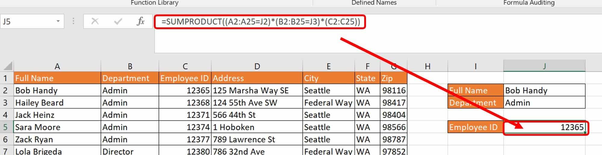
2. Type the following formula in cell J5:
=SUMPRODUCT((A2:A25=J2)*(B2:B25=J3)*(C2:C25))
The three innermost functions that Excel runs first are below:
A2:A25=J2
B2:B25=J3
C2:C25
Respectively, these three functions each virtually return the following array for Bob Handy in Admin:
{TRUE;FALSE;FALSE;FALSE;FALSE;FALSE;FALSE;FALSE;FALSE;FALSE;FALSE;FALSE;FALSE;FALSE;FALSE;FALSE;FALSE;FALSE;FALSE;FALSE;FALSE;FALSE;FALSE;FALSE}
{TRUE;TRUE;TRUE;TRUE;TRUE;FALSE;FALSE;FALSE;FALSE;FALSE;FALSE;FALSE;FALSE;FALSE;FALSE;FALSE;FALSE;FALSE;FALSE;FALSE;FALSE;FALSE;FALSE;FALSE}
{12365;12368;12371;12374;12377;12380;12383;12386;12389;12392;12395;12398;12401;12404;12407;12410;12413;12416;12419;12422;12425;12428;12431;12434}
These arrays are the result of Excel checking each row in the column identified and returning either TRUE or FALSE when the selected criteria is present. J2 has the full name Bob Handy in it, and Excel is looking for that name in each row of column A. The only row where Bob Handy appears is in position one of the 18 rows. Therefore, TRUE is the first number in the array, followed by 17 instances of FALSE.
By adding the AND (*) operator, Excel combines the first and second criteria, Full Name and Department and multiplies the results of their arrays, which renders the following virtual array:{1;0;0;0;0;0;0;0;0;0;0;0;0;0;0;0;0;0;0;0;0;0;0;0}
Next, Excel multiplies this array by the last array, which reports back the Employee ID. Altogether, the three functions result in the following: {12365;0;0;0;0;0;0;0;0;0;0;0;0;0;0;0;0;0;0;0;0;0;0;0}
This simply reports 12365.
You can also use SUMPRODUCT across multiple sheets. The function will sum the results with the correct address for the sheets written in the formula. This can be confusing for novice users because these formulas can get long, but taking them one piece at a time gives you the correct syntax. In the example above, if you were referencing data from another worksheet, you would have the additional single quotes and exclamation mark (‘Sheet name’!) before the table reference, such as:
For a different workbook, you would place the workbook name in brackets [Workbook name.xlsx] before the worksheet name reference.
How to Perform a Case-Sensitive Lookup in Excel Using EXACT
One issue with Excel’s VLOOKUP function is that it is not case-sensitive. You may have strings with both uppercase and lowercase text that serves to differentiate the content. For example, VLOOKUP reads the following data as the same:
- XMN2345-dl
- Xmn2345-Dl
- xmn2345-DL
Since you require unique values in VLOOKUP to return the correct value, use the EXACT function as a workaround for case-sensitivity requirements. The syntax for EXACT:
=EXACT(text1,text2)
The EXACT function compares two strings and returns TRUE if they are the same and FALSE if they are different.
Follow these steps to perform a case-sensitive lookup using EXACT.
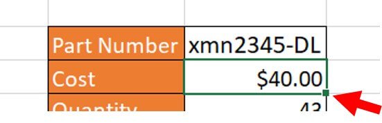
1. Click on the Exact Lookup worksheet tab in the VLOOKUP Advanced Sample file .
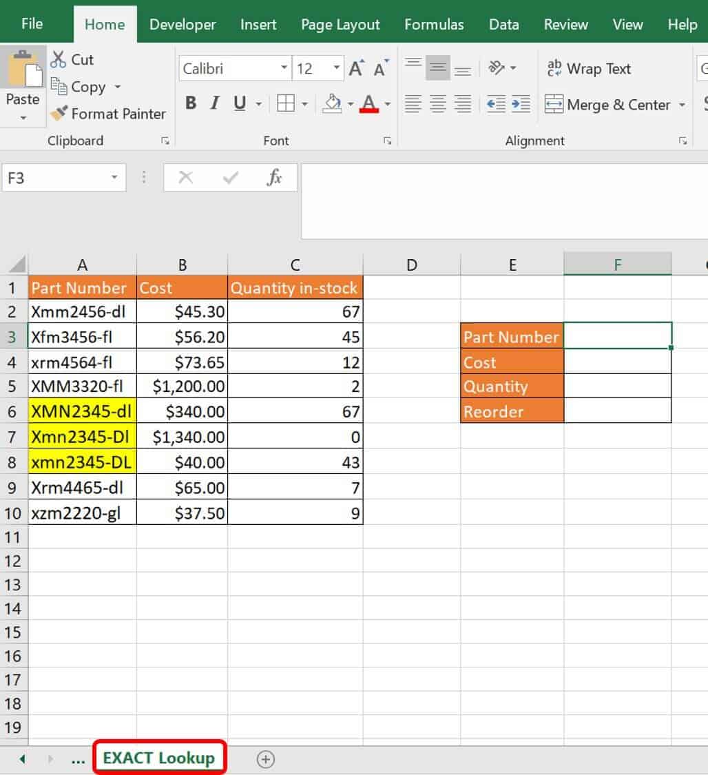
This worksheet has a data table with part numbers. Some of the part numbers appear to be the same except for the text case. To differentiate these in a lookup, wrap the LOOKUP with EXACT.
2. Type the following formula in cell F2, for the part number xmn2345-DL:
=LOOKUP(TRUE,EXACT($A$2:$A$10,$F$3),$B$2:$B$10)
Excel calculates the EXACT function first. The data in column A is compared to the value in F3 for the exact match, including the case. The virtual result:
{FALSE;FALSE;FALSE;FALSE;FALSE;FALSE;TRUE;FALSE;FALSE}
Only the seventh value matches the value in F3 exactly, so the seventh place in the array returns with TRUE. This value location is then added to the LOOKUP formula.
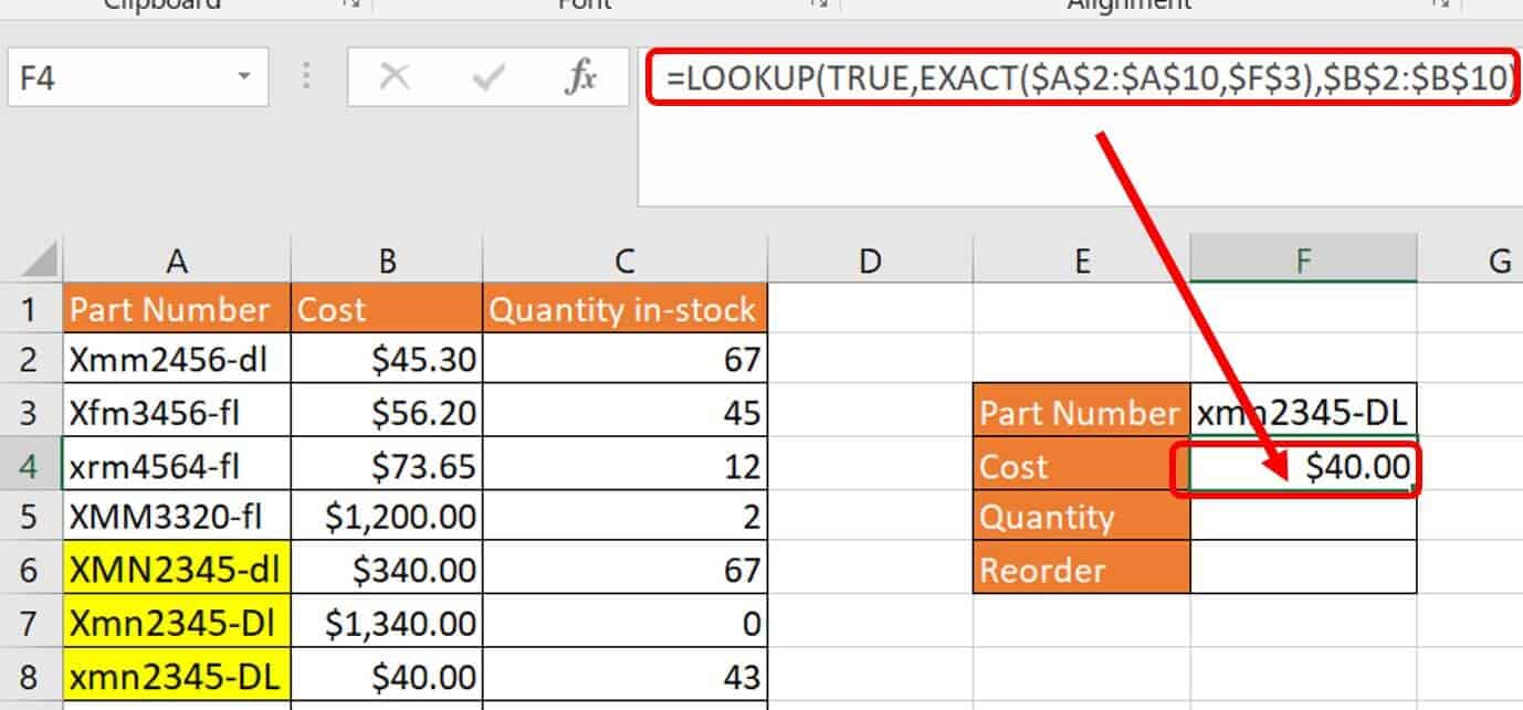
This is the primary usage of the LOOKUP formula:
=LOOKUP(lookup_value,lookup_vector, [result vector]
The return is the data that matches the TRUE location row in column B.
3. Type the following formula in cell F5:
=LOOKUP(TRUE,EXACT($A$2:$A$10,$F$3),$C$2:$C$10)
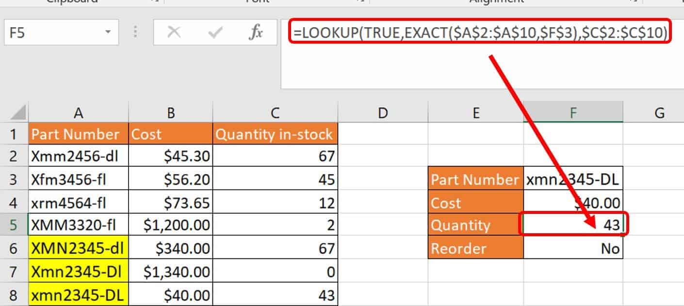
The return is the data that matches the TRUE location row in column C.
How to Look Up Data on Multiple Sheets
One challenge many people encounter is deciding how to use all these lookup functions to check different sheets and only return data if it is found. In other words, have Excel check worksheet number one; if the data is not there, check worksheet number two; if it is not there check worksheet number three; and so on. The good news is that you can perform this iterative process creatively.
Follow these steps to perform a lookup using multiple sheets.
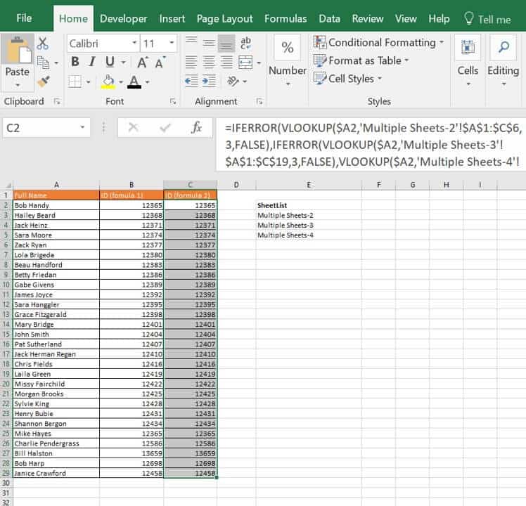
1. Click on the Multiple Sheets-1 worksheet tab in the VLOOKUP Advanced Sample file .
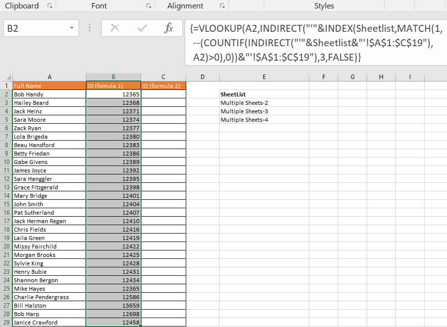
You will enter your formulas in this worksheet. In this example, there is a list of staff and you are looking for the data you need on several other worksheets in succession. As you can see, there are two columns for ID: ID (formula 1), and ID (formula 2). This example offers two separate formulas that you can use to perform this function. The first is more complex, but allows you to have a simple formula with a limited length by using the Excel task, Named Range.
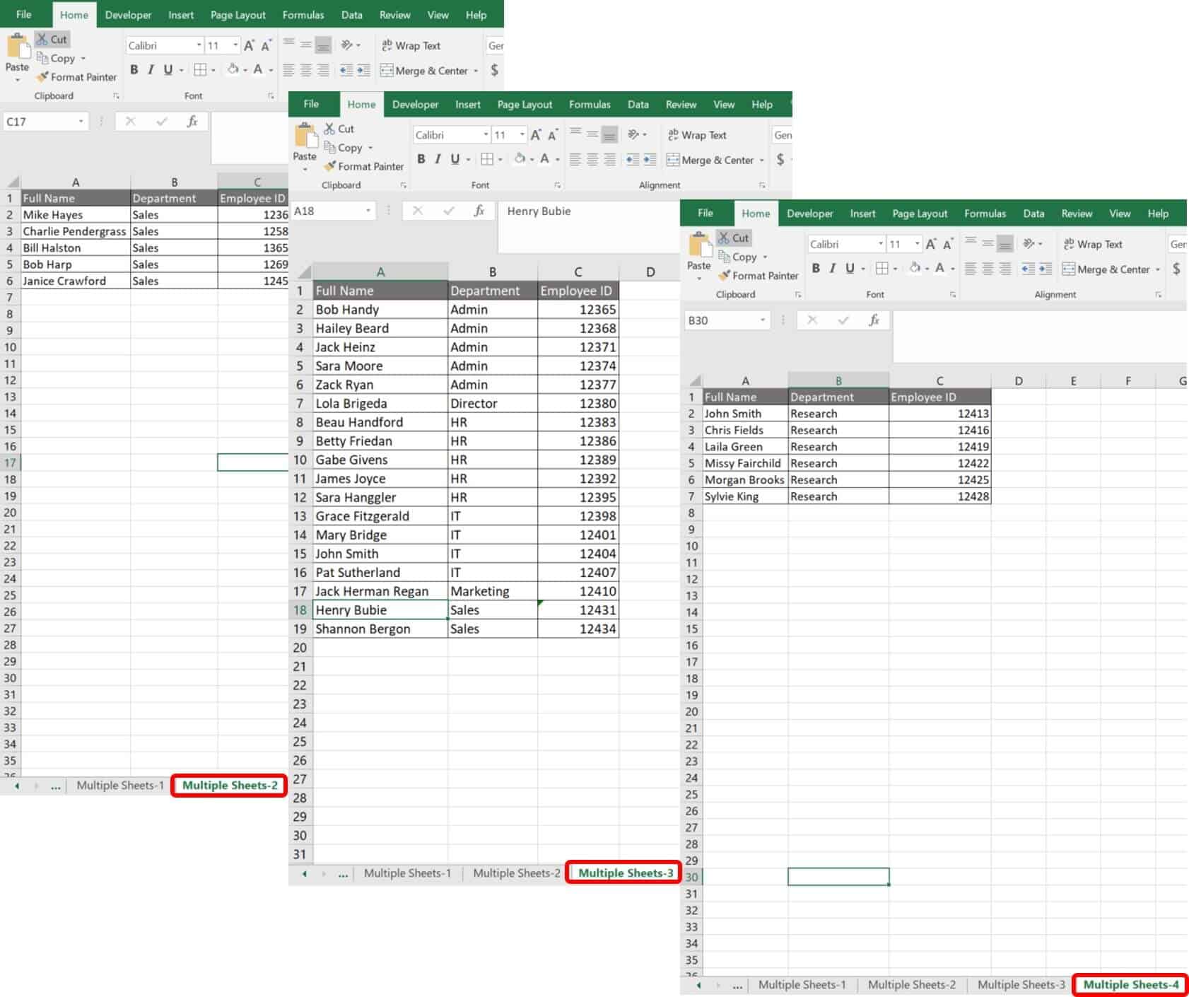
Multiple Sheets-2, Multiple Sheets-3, and Multiple Sheets-4 are the three worksheets you’ll use to draw the data. These worksheet names are listed on the first worksheet where you are compiling your formulas, Multiple Sheets-1. Together, they have been named Sheetlist.
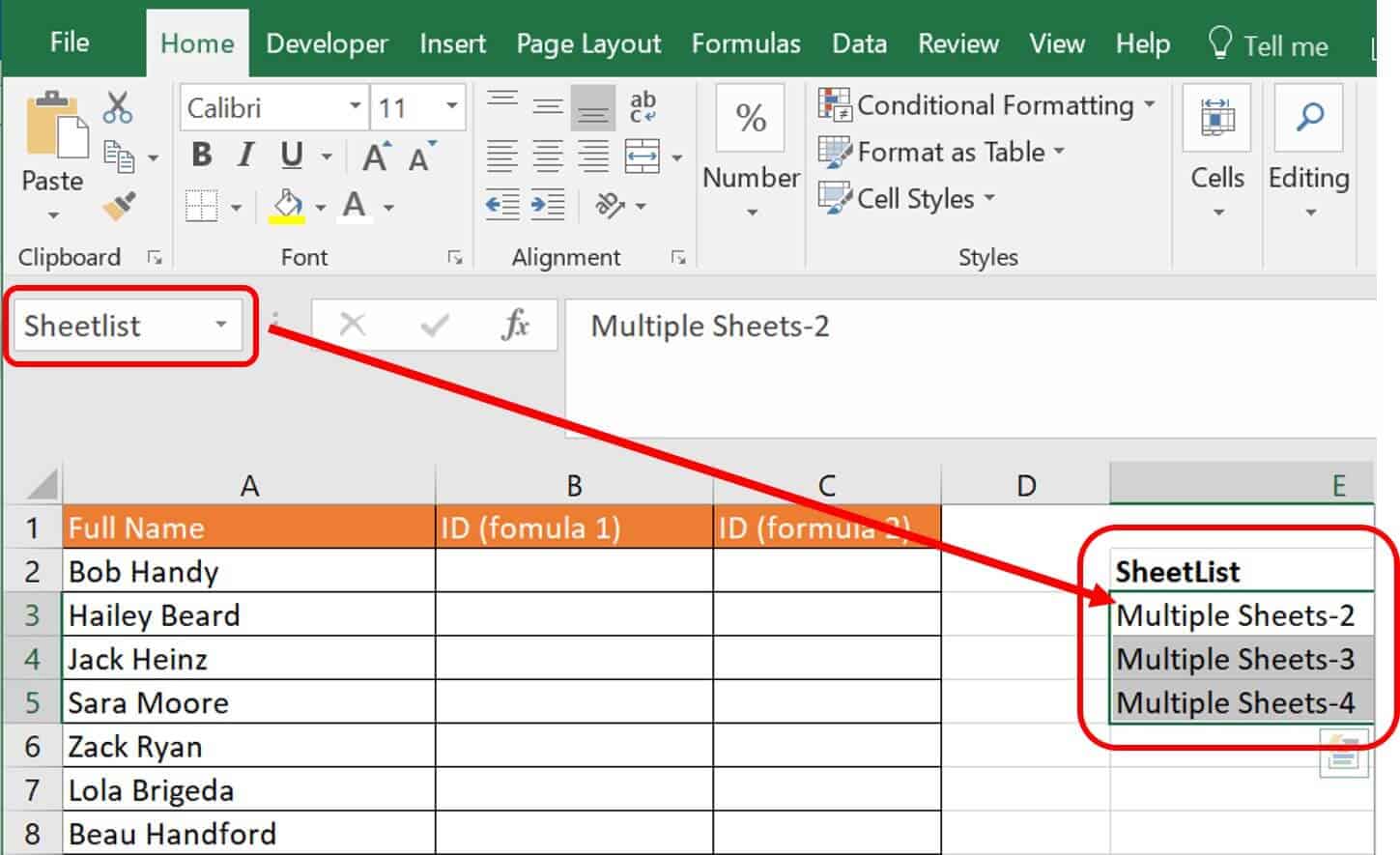
We used the Named Range function in Excel to create this sheet list. To perform this task, simply highlight the list of cells with the names and enter a name (in this scenario we entered Sheetlist), which gives you a named range of cells. However, Excel’s nomenclature rules require that you do not use spaces, non-alphanumeric characters, or underscores in a named range title.
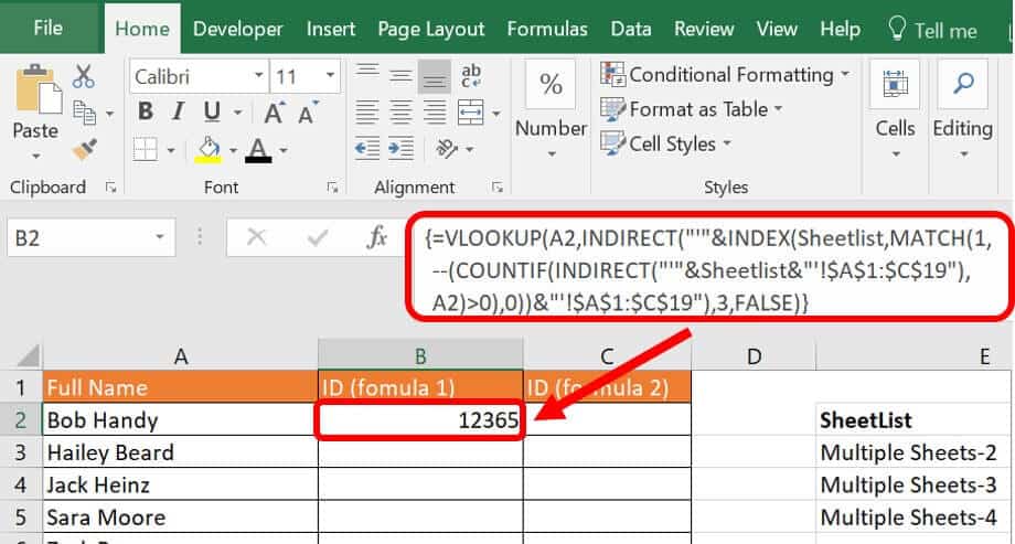
2. Type the following formula in cell B2 on the Multiple Sheets-1 worksheet:
=VLOOKUP(A2,INDIRECT("'"&INDEX(Sheetlist,MATCH(1,--(COUNTIF(INDIRECT("'"&Sheetlist&"'!$A$1:$C$19"),A2)>0),0))&"'!$A$1:$C$19"),3,FALSE)
3. Click Ctrl+Shift+Enter on your keyboard to turn this formula into an array.
This formula uses VLOOKUP, INDIRECT, INDEX, and COUNTIF to look through the defined list of worksheets.
The first formula that Excel calculates is the INDIRECT function:
=INDIRECT("'"&Sheetlist&"'!$A$1:$C$19")
INDIRECT returns a reference to a range. When calculated this function returns the following:
{"Full Name";"Full Name";"Full Name"}
The next function calculated is the COUNTIF function:
=COUNTIF(INDIRECT("'"&Sheetlist&"'!$A$1:$C$19"),A2)>0)
The result of this formula:
({FALSE;TRUE;FALSE})
When Excel searches for the value in cell A2 (Bob Handy) in the three worksheets, it will return either TRUE or FALSE. In this scenario, the value is found in the second worksheet searched, Multiple Sheets-3.
Next is the MATCH function, which calculates the following:
MATCH(1,--(COUNTIF(INDIRECT("'"&Sheetlist&"'!$A$1:$C$19"),A2)>0),0)
The MATCH function returns the position in the array — in this case, 2.
The INDEX function is next:
INDEX(Sheetlist,MATCH(1,--(COUNTIF(INDIRECT("'"&Sheetlist&"'!$A$1:$C$19"),A2)>0),0))
From this formula, Excel returns Multiple Sheets-3.
Another INDIRECT function is calculated, and the formula is the following:
INDIRECT("'"&INDEX(Sheetlist,MATCH(1,--(COUNTIF(INDIRECT("'"&Sheetlist&"'!$A$1:$C$19"),A2)>0),0))&"'!$A$1:$C$19")
This formula returns the following:
{"Full Name","Department","Employee ID";"Bob Handy","Admin",12365;"Hailey Beard","Admin",12368;"Jack Heinz","Admin",12371;"Sara Moore","Admin",12374;"Zack Ryan","Admin",12377;"Lola Brigeda","Director",12380;"Beau Handford","HR",12383;"Betty Friedan","HR",12386;"Gabe Givens","HR",12389;"James Joyce","HR",12392;"Sara Hanggler","HR",12395;"Grace Fitzgerald","IT",12398;"Mary Bridge","IT",12401;"John Smith","IT",12404;"Pat Sutherland","IT",12407;"Jack Herman Regan","Marketing",12410;"Henry Bubie","Sales",12431;"Shannon Bergon","Sales",12434}
Finally, the VLOOKUP is calculated. Here is the formula:
=VLOOKUP(A2,{"Full Name","Department","Employee ID";"Bob Handy","Admin",12365;"Hailey Beard","Admin",12368;"Jack Heinz","Admin",12371;"Sara Moore","Admin",12374;"Zack Ryan","Admin",12377;"Lola Brigeda","Director",12380;"Beau Handford","HR",12383;"Betty Friedan","HR",12386;"Gabe Givens","HR",12389;"James Joyce","HR",12392;"Sara Hanggler","HR",12395;"Grace Fitzgerald","IT",12398;"Mary Bridge","IT",12401;"John Smith","IT",12404;"Pat Sutherland","IT",12407;"Jack Herman Regan","Marketing",12410;"Henry Bubie","Sales",12431;"Shannon Bergon","Sales",12434},3,FALSE)
The return from this formula is 12365.
3. Copy and drag this formula down through cell B29.
This formula will stay the same regardless of how many sheets you type into the Sheetlist, making it finite.
To perform the same function with another formula, type the following formula into cell C2:
=IFERROR(VLOOKUP($A2,'Multiple Sheets-2'!$A$1:$C$6,3,FALSE),IFERROR(VLOOKUP($A2,'Multiple Sheets-3'!$A$1:$C$19,3,FALSE),VLOOKUP($A2,'Multiple Sheets-4'!$A$1:$C$16,3,FALSE)))
This formula performs a VLOOKUP for every worksheet and wraps them with IFERROR functions. A VLOOKUP is necessary for each worksheet.
This formula can become long and onerous if you’re entering many worksheets.
How to Perform a Lookup of Multiple Values in Google Sheets
Google Sheets, Excel’s competitor, operates solely in the cloud and has many of the same functions as Excel. Many of these functions convert between the two programs, but they are not able to pull data cross-program for specific formulas.
Follow these steps to perform a lookup and return matching values horizontally in Google Sheets.
1. Click on the Multiple values-horizontal in the worksheet tab in the Google Sheets sample file.
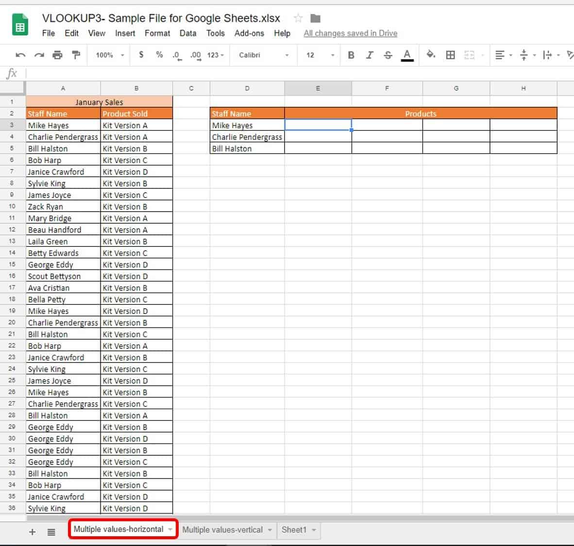
This worksheet has a list of staff names and the products they sold in January. In this example, we want to horizontally list the products sold by three staff members. Here’s the original formula used in Excel:
{=IFERROR(INDEX($B$3:$B$37,SMALL(IF(D$3=$A$3:$A$37,ROW($B$3:$B$37)-2,""), COLUMN()-4)),"")}
In Google Sheets, this formula becomes:
=ARRAY_CONSTRAIN(ARRAYFORMULA(IFERROR(INDEX($B$3:$B$37,SMALL(IF($D3=$A$3:$A$37,ROW($B$3:$B$37)-2,""), COLUMN()-4)),"")), 1, 1)
Google calls out the Array requirements with its own syntax (ARRAY_CONSTRAINTS and ARRAYFORMULA). Also, you do not need to press Ctrl+Shift+Enter on your keyboard to create an array.
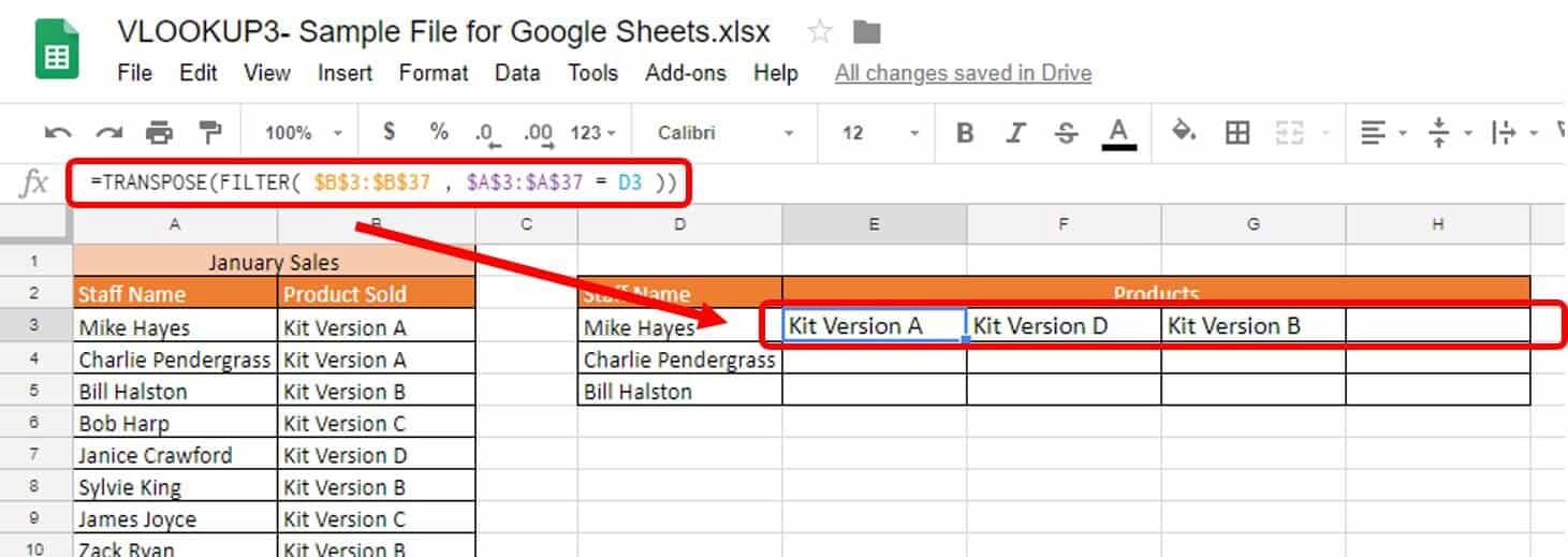
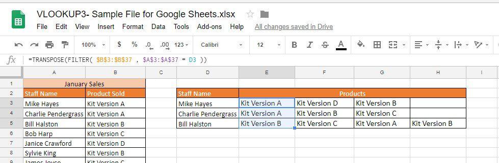
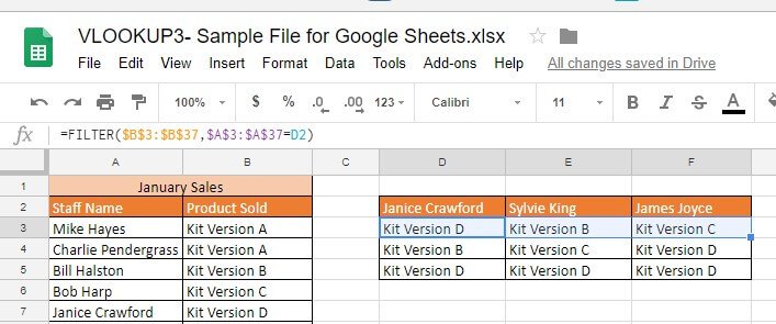
2. Try an easier and less complicated formula for this same result. Type the following formula in cell E3:
=TRANSPOSE( FILTER( $B$3:$B$37 , $A$3:$A$37 = D3 ) )
Although the exercise is the same as the Excel version for horizontal returns, this is quite a different formula. It is much simpler in Google Sheets because of the powerful FILTER function, which is not available in Excel. FILTER returns the specified range of rows or columns that meet the criteria. The syntax for FILTER is:
=FILTER(range, condition1, [condition2],…)
Breaking down this formula, the first function that Google Sheets performs is FILTER:
Argument | Value | Meaning |
Range | B3:B37 | The column of data to return. |
Condition1 | A3:A37=D3 | The criteria that provides a TRUE/FALSE and limits the return. |
In other words, this FILTER function looks at each entry in the column and returns it if it is deemed TRUE. This is the case if the entry next to it is equal to D3. Without the TRANSPOSE part of the formula, this return would be vertical, not horizontal. Adding TRANSPOSE completes this to a horizontal return.
3. Select and drag cell E3 down through cells E4 and E5 to automatically load the formulas.
Follow these steps to perform VLOOKUP and return all matching values vertically in Google Sheets.
1. Click on the Multiple values_row worksheet tab in the Google Sheets sample file.

The original Excel formula was:
=IFERROR(INDEX($B$3:$B$37,SMALL(IF(D$2=$A$3:$A$37,ROW($B$3:$B$37)-2,""), ROW()-2)),"")
In Google Sheets, this formula becomes:
=ARRAY_CONSTRAIN(ARRAYFORMULA(IFERROR(INDEX($B$3:$B$37,SMALL(IF(D$2=$A$3:$A$37,ROW($B$3:$B$37)-2,""), ROW()-2)),"")), 1, 1)
Google Sheets adds the extra array functions to compensate for not using the traditional curly brackets seen in Excel.
2. Use an easier formula in Google Sheets, and type the following in cell D3:
=FILTER($B$3:$B$37,$A$3:$A$37=D2)
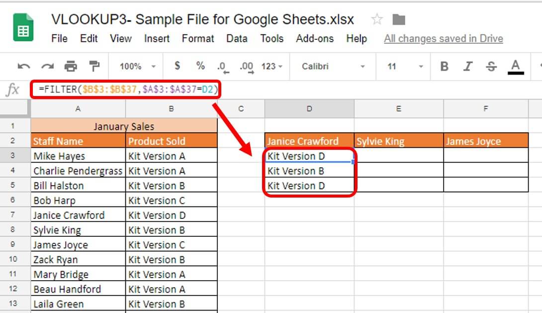
This one simple function performs this return.
3. Select and drag cell D3 through cells E3 and F3. All data loads into your chart.
Connect Data Across Your Work with VLOOKUP in Smartsheet
Empower your people to go above and beyond with a flexible platform designed to match the needs of your team — and adapt as those needs change.
The Smartsheet platform makes it easy to plan, capture, manage, and report on work from anywhere, helping your team be more effective and get more done. Report on key metrics and get real-time visibility into work as it happens with roll-up reports, dashboards, and automated workflows built to keep your team connected and informed.
When teams have clarity into the work getting done, there’s no telling how much more they can accomplish in the same amount of time. Try Smartsheet for free, today.