How to Make a Gantt Chart in Google Sheets Using a Template
To create a Gantt chart in Google Sheets, download a Gantt chart template from this page, and follow the steps below. This step-by-step guide provides details on how to open and complete the Gantt chart template.
- Open the Template
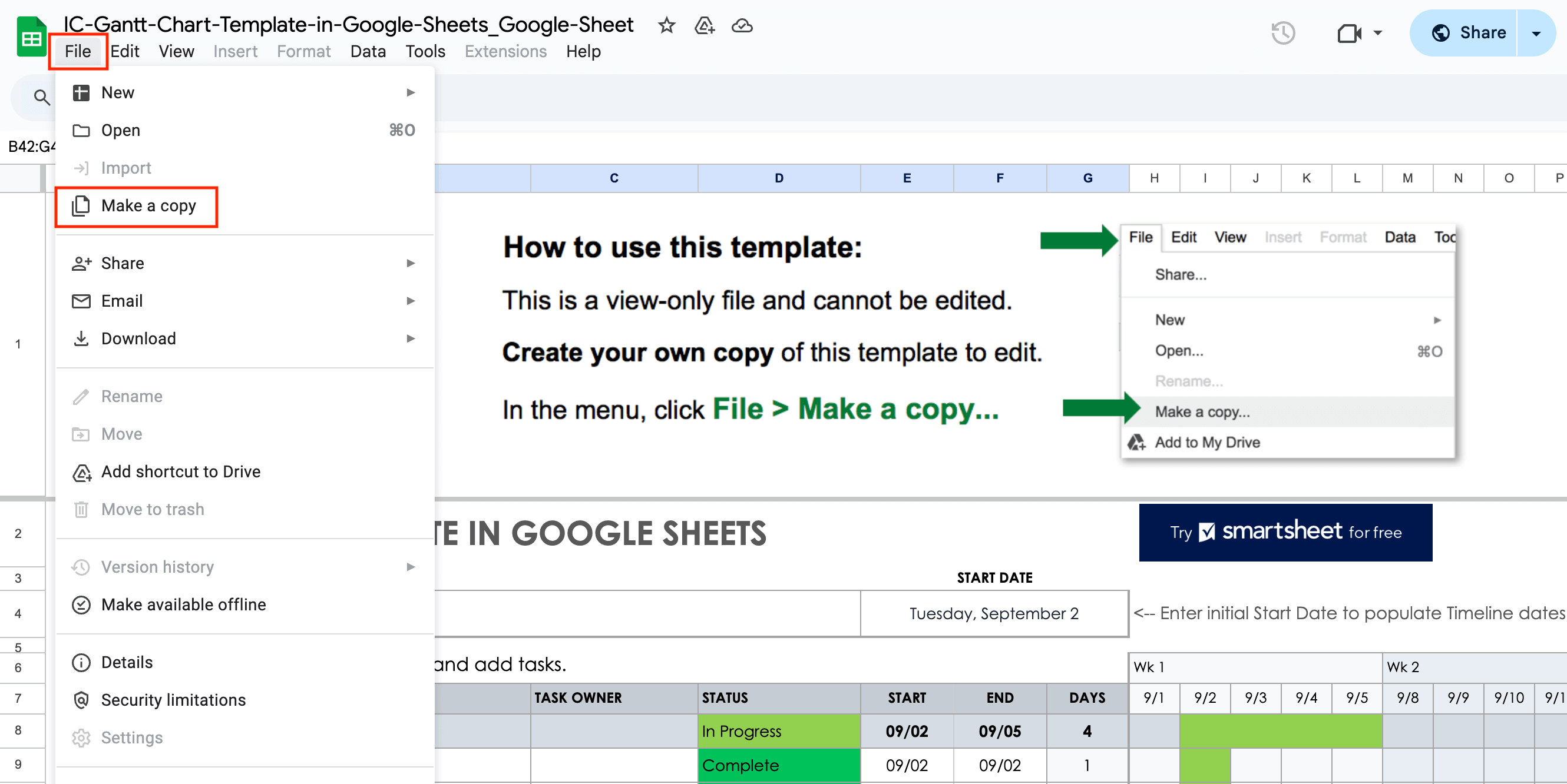
Open the Gantt chart template in Google Sheets.
- Make a Copy
Click File > Make a copy to make an editable copy of the template.
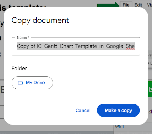
Name the document, select a folder, and click Make a copy.
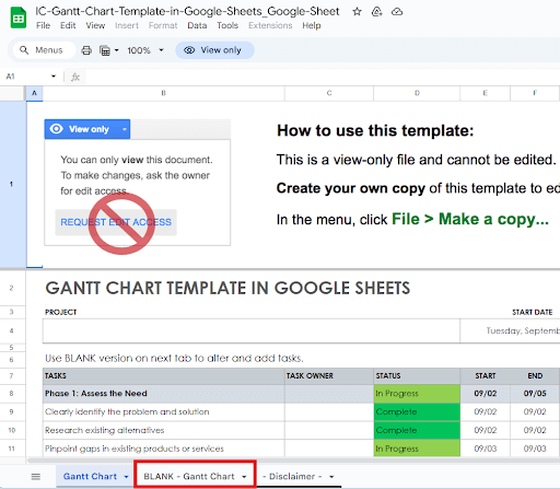
Once the template opens, click on the the BLANK - Gantt Chart tab at the bottom of the sheet.
- Enter the Project Name and Start Date
In the Project field, enter the project’s name and a brief description. In the Start Date field, enter the project’s start date.

- Enter Project Details
Enter project tasks, task owners, status, and start and end dates.

Once you enter a start and end date for each task, the template will auto-populate a duration bar on the right-hand side of the template.
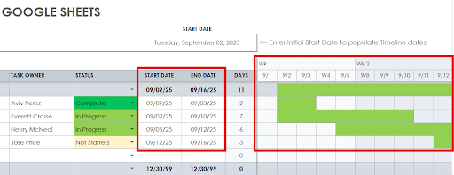
The template also calculates the number of days to complete the task under the Days column.

To learn more about Gantt charts, including their history and why they’re a beneficial tool for project management, visit this article about Gantt charts.
Video: Create a Gantt Chart with a Google Sheets Template

How to Make a Gantt Chart in Google Sheets
A Gantt chart in Google Sheets uses horizontal bars to represent the duration of each task. A Gantt chart enables you to track your progress, task dependencies, and key milestones. Follow the steps below to quickly create a Gantt chart with Google Sheets.
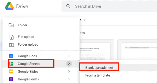
- Open a New Google Sheets Spreadsheet
Click New > Google Sheets > Blank spreadsheet.

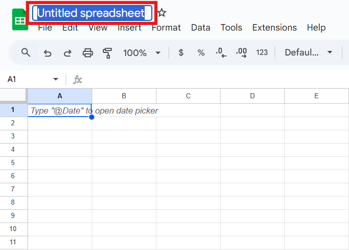
- Rename the Document
Name the document by replacing the placeholder text with the name of your project.
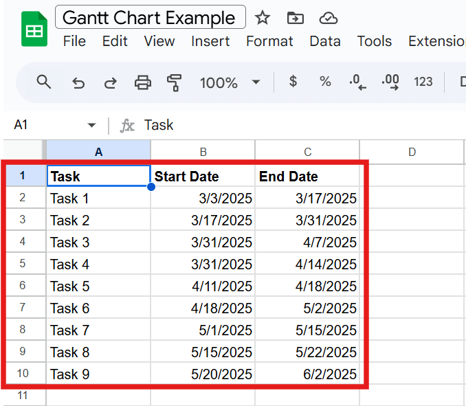
- Enter Project Data
To enter project data for the Gantt chart, you’ll need to make two tables. The first table serves as a template for the calculations you create in the second table.
For the first table, enter column data for your project tasks, along with their start and end dates.
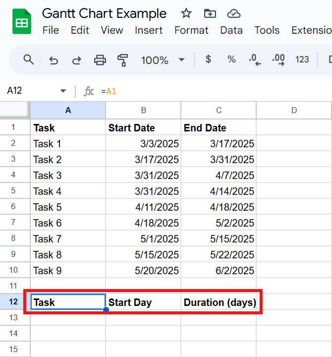
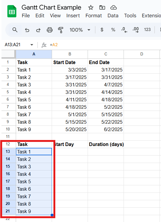
Create the second table a few rows below the first one. Enter Task, Start Day, and Duration (days) column headings.
Tip: The task lists in both tables should be identical. Copy the tasks from the first table and paste them into the second table.
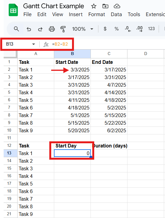
- Enter the Start Day Formulas
Determine the start day for each task. The Start Day for Task 1 is 0 (this will serve as the starting point for all task durations). Enter a formula for Start Date - Start Date. In the example below, it is =int(B2)-int(B2).
To determine the remaining Start Day values, enter a formula to find the difference between each task’s start date and that of the first task: Task 1’s Start Date - Task 2’s Start Date. In the example below, it is =int(B3)-int(B2).
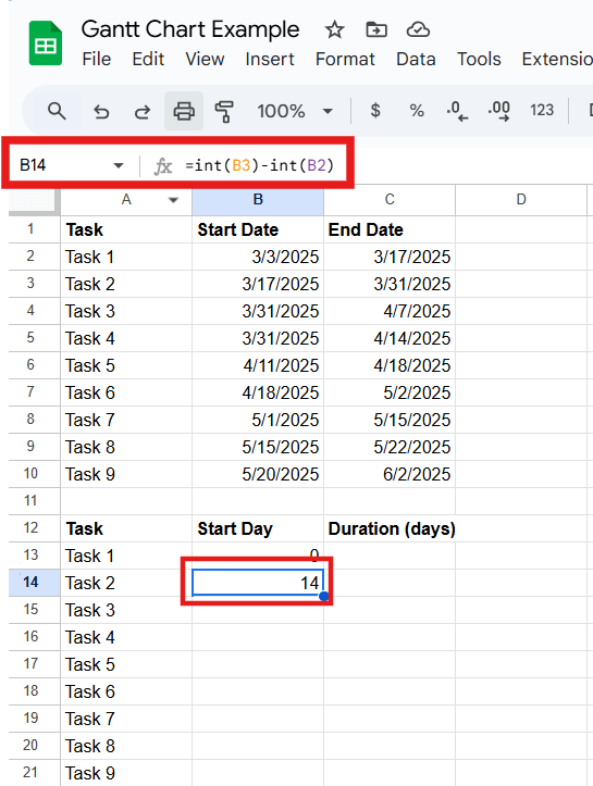
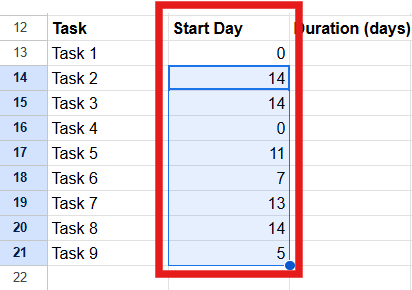
Click Task 2’s Start Day cell, and drag the small blue box in the bottom-right corner of the cell until you reach the last project task. The remaining tasks’ start days will auto-populate.
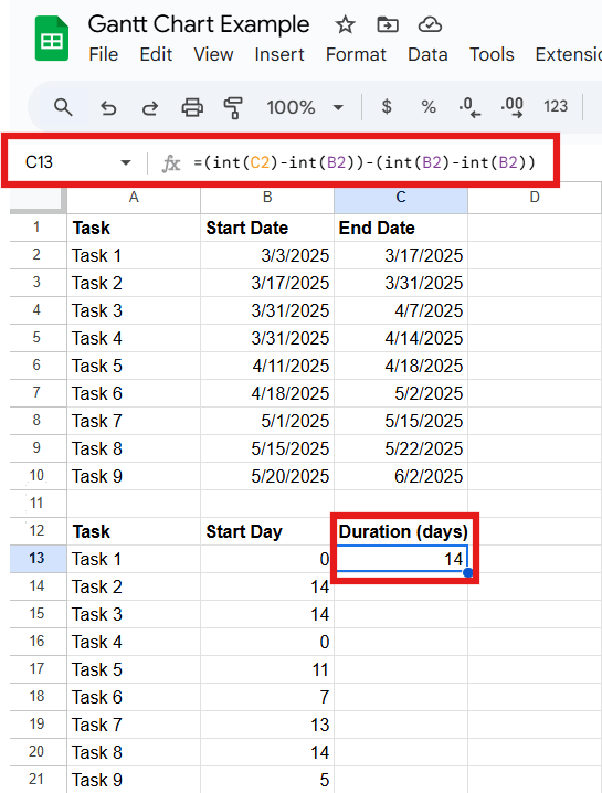
- Enter the Duration Formulas
To determine the duration of each task, subtract each task’s start date from the end date and subtract the start date from the start date. In the example below, the formula is =(int(C2)-int(B2))-(int(B2)-int(B2)).
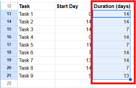
Click the Duration cell for Task 1, and drag the small blue box in the bottom-right corner of the cell until you reach the last project task. The durations of the remaining tasks will auto-populate.
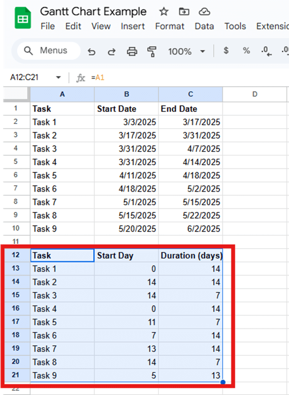
- Create a Stacked Bar Graph
Highlight the second table. The highlighted data will be used for the chart.
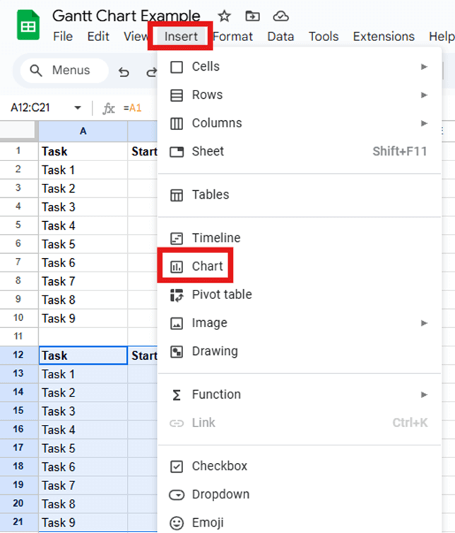
Click Insert > Chart. A stacked bar chart will appear on the page.
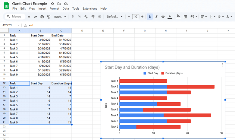
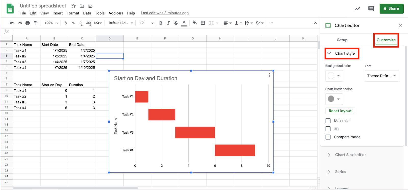
- Convert the Stacked Bar Graph to a Gantt Chart
Click on any Start Day bar in the chart to highlight all the Start Day bars. In the example below, this is the blue portion of the bars.
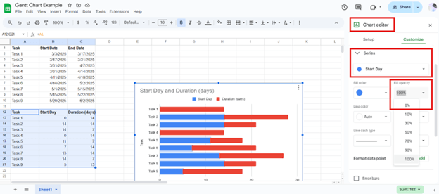
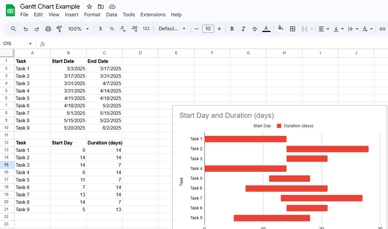
In the Chart editor panel on the right, click the Customize tab. Click Series, then click the drop-down menu and Start Day. Under Fill opacity, click 0%. The chart should now resemble a Gantt chart.
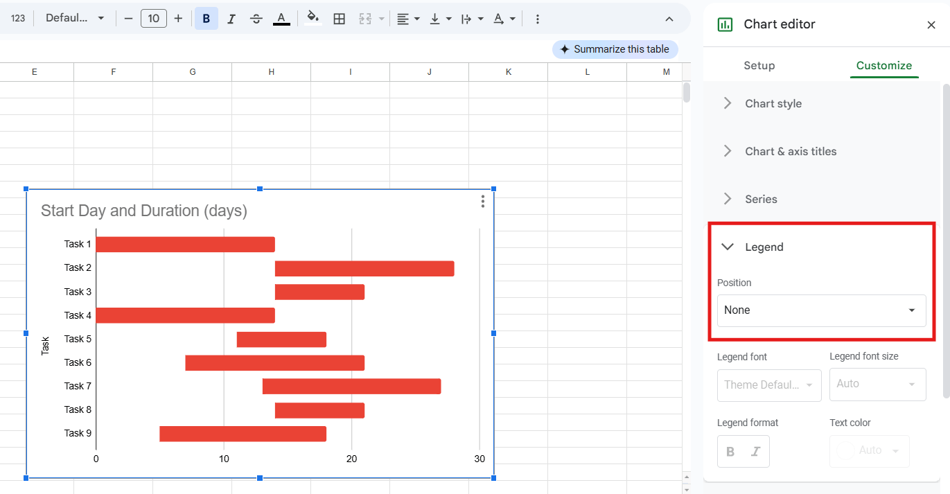
Tip: To remove the legend, select None from the Legend drop-down menu in the Chart editor.
Use Google Sheets daily schedule templates and planners to improve your day-to-day productivity.
Tips for Customizing a Gantt Chart in Google Sheets
It’s easy to customize your Gantt chart using the Chart editor. You can customize the chart title, the style of the bars, the bar colors, the axes labels, and more. Below, you’ll find tips and how-tos to customize the chart to fit your needs.
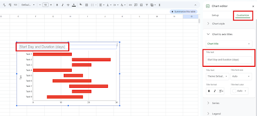
Update the Gantt Chart Title
Double-click the chart to open the Chart editor menu on the right. Click the Customize tab and Title text. Type in a new title, and press Enter.
Customize the Gantt Chart Area
Follow these steps to change the appearance of your chart by adjusting the border color or making the bars pop in 3D.
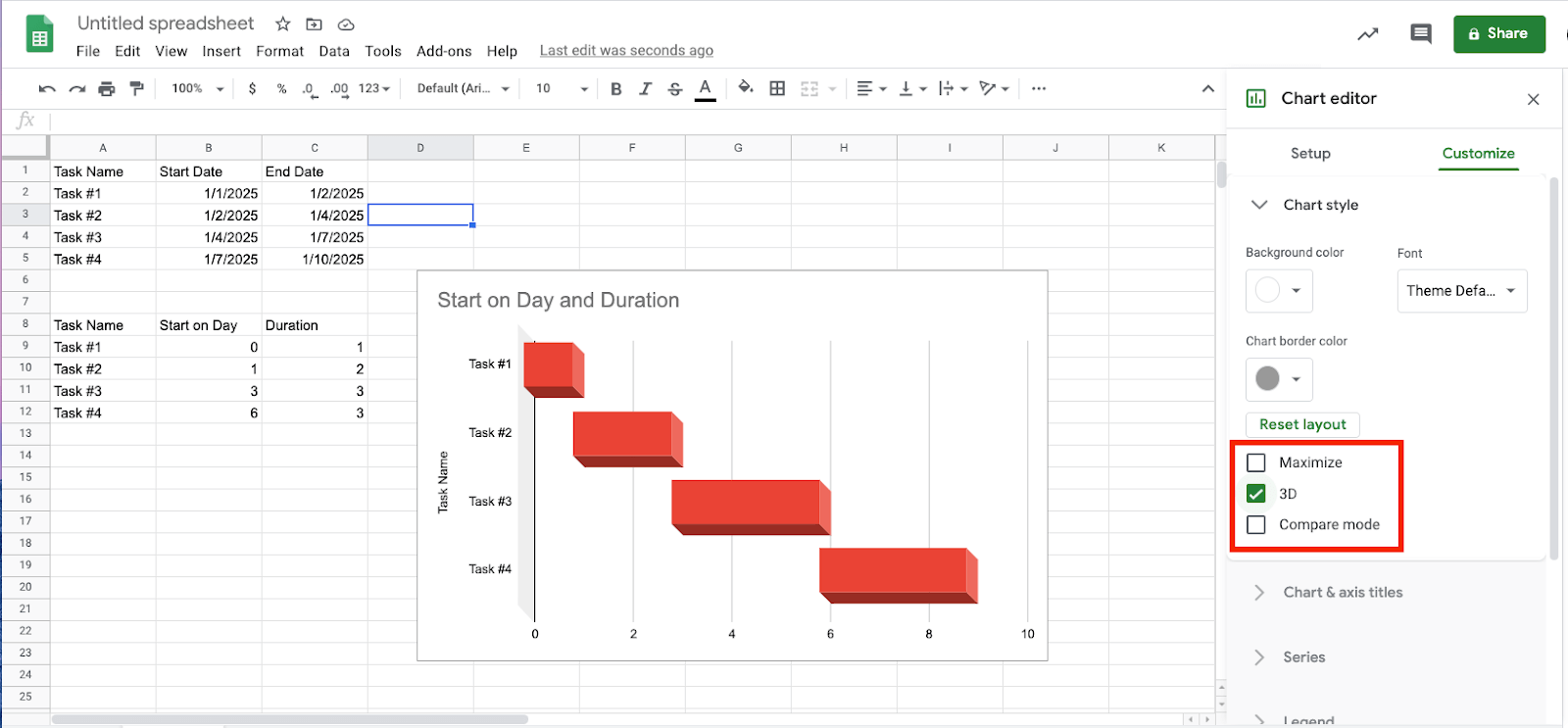
- Double-click the chart and navigate to the Chart editor menu on the right.
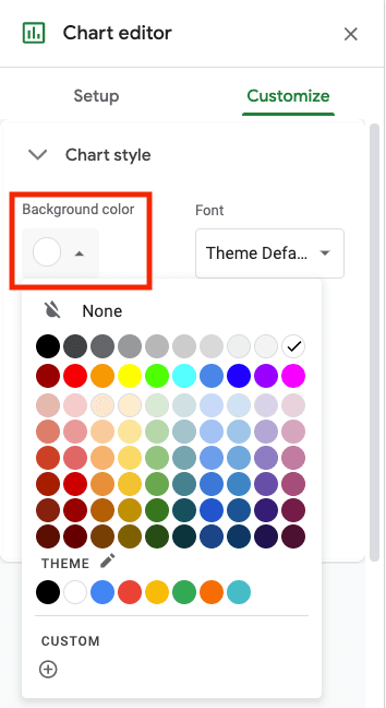
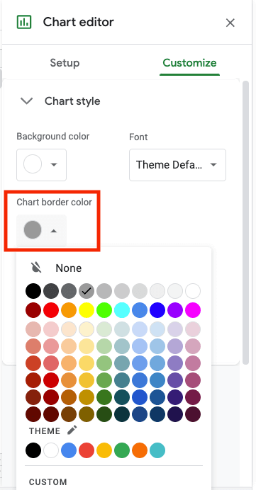
- Click the Customize tab, then click Chart style.
- Click the drop-down menu under Background color, then click a color to change the background color.
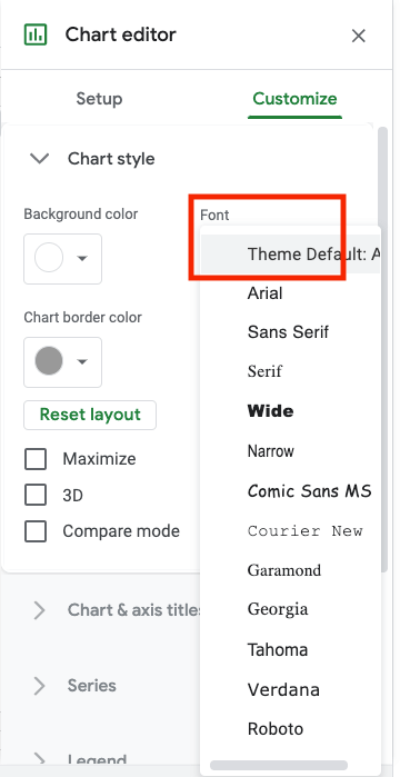
- Click on the text you want to change in the chart. Click the Font drop-down menu to change the font style for labels, legends, or the title.
Note: You need to click on the text type to make changes.
- Click the Chart border color drop-down menu. Click a border or color, or click None to remove it completely.
- Click the 3D box to add the effect to the bars.
Learn the unique benefits of Gantt view in Smartsheet and find a step-by-step video in this guide on how to create a Gantt chart in Smartsheet.
How to Handle Gantt Charts With Dependencies in Google Sheets
To create dependencies between tasks in Google Sheets, first identify which tasks can’t start until a previous task or series of tasks is complete. Then, add a formula to set the dependency, or add formulas to show tasks that can happen concurrently. Below, you’ll find a step-by-step guide for setting up task dependencies.
- A task dependency is a task that can only be completed once another task is done. Determine the task dependencies in your project, including the tasks they depend on.
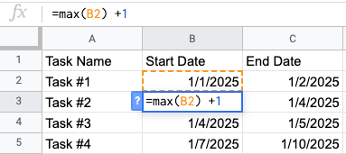
- In the first table, click the cell of the dependent task.
- In the Start Date cell of the dependent task, type in this formula:
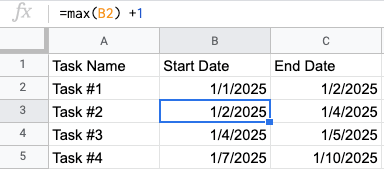
=max(B2)+1
Tip: The +1 signifies this task can only start the day after the other tasks in the formula are completed.
The resulting value in the dependent task cell should be the date after the other tasks in the formula are projected to be completed.
Check out our roundup of project management templates in Google Sheets to standardize your project management process. If you’re looking for templates that help you track task details and their status, check out this collection of Google Sheets project tracker templates.
How to Export a Gantt Chart in Google Sheets to Excel
Some people prefer working in a more familiar spreadsheet interface, such as Microsoft Excel. Follow these steps to export a Gantt chart and all corresponding project data in Google Sheets to Excel.
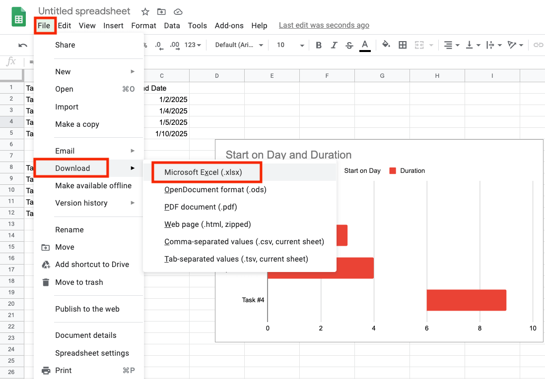
- Click File and scroll down to Download.
From the Download drop-down menu, click Microsoft Excel (.xlsx).
Use this action to automatically create and download an Excel file.
Follow this tutorial to learn how to make a Gantt Sheet in Excel.

Use Smartsheet to Create a More Powerful and Useful Gantt Chart
Empower your people to go above and beyond with a flexible platform designed to match the needs of your team — and adapt as those needs change.
The Smartsheet platform makes it easy to plan, capture, manage, and report on work from anywhere, helping your team be more effective and get more done. Report on key metrics and get real-time visibility into work as it happens with roll-up reports, dashboards, and automated workflows built to keep your team connected and informed.
When teams have clarity into the work getting done, there’s no telling how much more they can accomplish in the same amount of time. Try Smartsheet for free, today.
Google Sheets Gantt Chart FAQs
Google Sheets makes it easy to build, share, and update Gantt charts for smaller or midsize projects. It offers real-time access and flexible design, and it works on any device. You can link data, use formulas, and collaborate without extra tools or downloads.
Below are some benefits of using Google Sheets to create Gantt charts:
- You can build a custom chart from scratch or start with a free template to save time.
- Google Sheets supports formulas, so your dates, durations, and percent complete update automatically.
- Team members can view or edit simultaneously with built-in sharing tools.
- Comments and notes help you track updates or decisions for each task.
- Google Sheets stores charts in the cloud so that you can access them anytime from any device.
Google Sheets works well for basic Gantt charts but lacks advanced tools. For example, task dependencies don’t update automatically, and there are no automated workflows. It lacks native tools for reporting on complex work, such as the ability to roll up reports into a dashboard.
Smartsheet offers built-in dashboards, reports, and automated workflows that provide better visibility, easier tracking, and smarter updates without extra setup or manual effort.
Google does not have a Gantt chart maker or a built-in Gantt chart template. To manually create a Gantt chart in Google, enter your project details (tasks, start, and end dates), highlight the data, and insert a chart. Use the chart editor panel to customize the look and feel of your Gantt chart. You can also download a template and reuse it for future projects.
Google Sheets does not have a prebuilt table with duration bars for Gantt charts. However, you can manually create a Gantt chart in Google Sheets using a stacked bar chart. Add custom formatting to represent task durations.
Smartsheet offers a Gantt chart template in Google Sheets that automatically creates duration bars for tasks with start and end dates. Use this customizable template to track project timelines without manually creating bars or conditional formatting.
Check out this complete collection of Google Sheets Gantt chart templates to help you visualize project overviews, manage tasks, and track progress.
You can find free, easy-to-use Google Sheets Gantt chart templates on Smartsheet. These templates help you plan and manage tasks, track timelines, and collaborate. They simplify work, align your team, and support short and long-term projects.
See how Gantt chart software can help you visualize project planning, manage tasks, dependencies, and track milestones and overall progress.
To make a monthly Gantt chart in Google Sheets, navigate to the Chart editor and click the Customize tab. Expand Gridlines and ticks, and set the horizontal axis to Major step to 30. Add a horizontal axis title under the chart. Enter Days in the Title text box and add titles to the Axis.
Making a timeline in Google Sheets is similar to creating a bar chart. Enter your project data (tasks, assignees, start dates, due dates), and insert a timeline using the timeline feature. You can customize which data you want displayed in the timeline view and color-code the cards.
Learn how to make a timeline in Google Docs, and check out pre-formatted timeline templates in Google Sheets, Docs, and Slides.

